Individual income can grow as fast as productivity rises.
Alex Berenson
Economics is the study of how consumers maximize utility, how producers maximize profit, how governments maximize welfare of their citizens and how investors maximize return. The law of diminishing returns gives us that for every unit of additional output produced, the addition to total cost increases more rapidly. Therefore, in perfect competition the supply curve is a positively sloped curve that as output increases is steeper. When we ask the firms how much they are willing to produce at different prices we derive the supply curve done in an empirical fashion. Perfect competition, monopoly, monopolistic competition, oligopoly comprise the economy and are all added up to define the short run aggregate supply curve (s.r.a.s.c.). In this essay some of the effects of changes in aggregate demand(A.D.) are taken into consideration. When the marginal cost curve shifts the s.r.a.s.c. shifts. In the long run, buildings and machinery increase but so do the wages therefore the long run aggregate supply curve (l.r.a.s.c.) is vertical at national income of full employment Y. At liquidity trap the A.D. is vertical, we prove it as this essay unfolds, resulting in sluggish economic growth or if the s.r.a.s.c. does not meet the A.D. in negative economic growth and negative inflation. It is proved that all short run supply curves are valid at price equal or greater than the average variable cost (A.V.C.). Finally, we tackle economic problems of countries such as liquidity trap, inflationary pressures and try to solve them. The solutions are suggestions.
Marginal cost
Profit maximization
Technical information 1
Perfect competition
Monopoly
Technical information 2
Monopolistic competition
Oligopoly
Adding up all markets
An example with figures
When A.D. increases
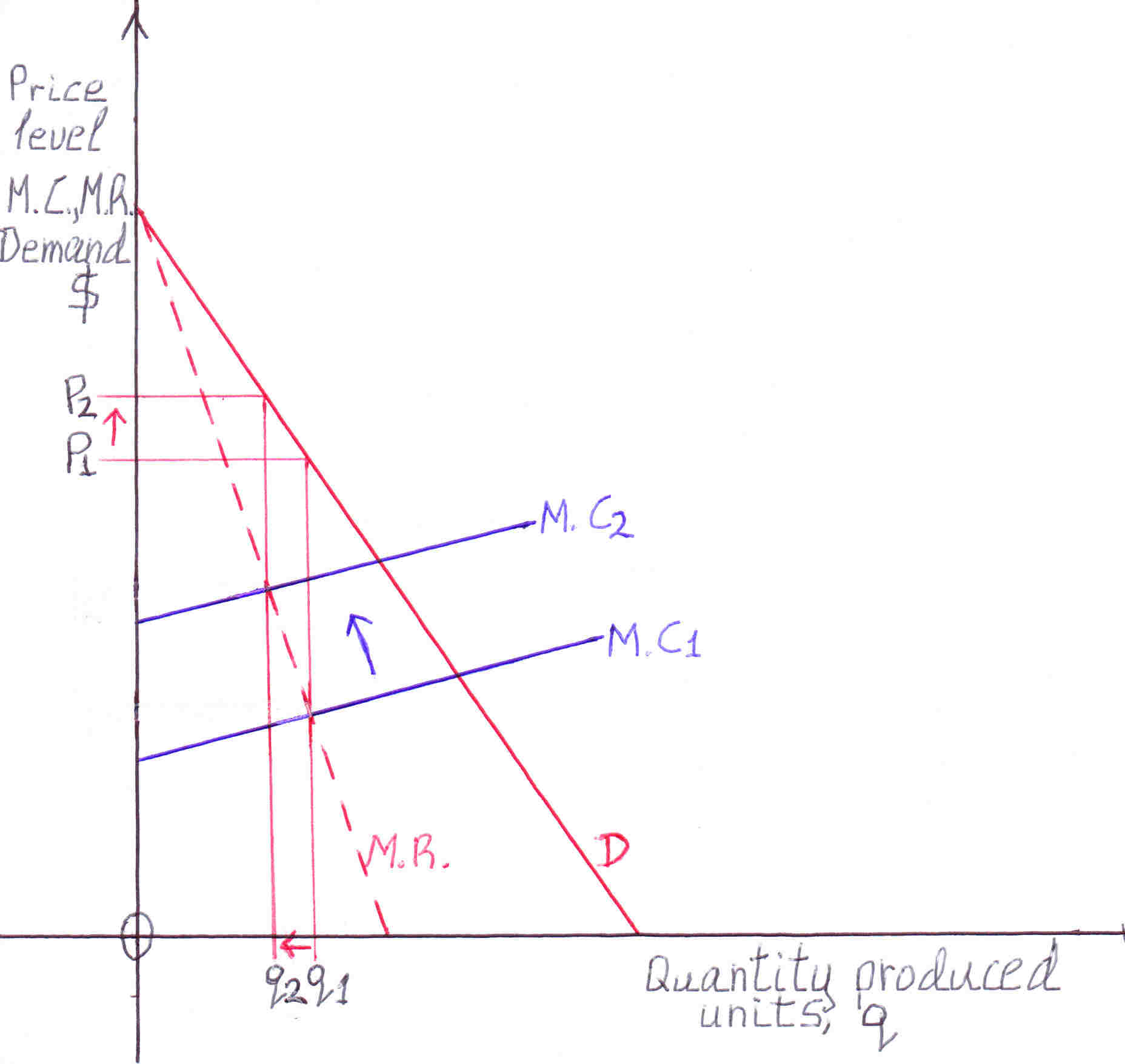
When marginal cost changes
Shape of the s.r.a.s.c.
l.r.a.s.c. is vertical
Liquidity trap
A.V.C. ≤ price, for production
When s.r.a.s.c. does not meet A.D.
Liquidity trap
l.r.a.s.c. shifts
Tight fiscal policy
Combat inflation
Deficit financing
A.D. > Aggregate Supply
Monthly payment of a loan
Marginal cost
Marginal cost(M.C.) is the cost incurred in producing one additional unit of output. It is the addition to Total cost(T.C.) for producing 1 additional unit of output. The law of diminishing returns gives us that the marginal cost increases at a faster pace. Why?
When we add input to produce more goods, for example, when we add workers (labor) there comes a time that the output does not increase by the same proportion of the additional labor employed. Too many workers collide, their relative space decreases they are more disorganized. The output they produce is not proportional to the input of labor. For example, a factory building with the machines has a capacity of 100 workers if the workers are increased to 200 the output will not double. Workers are not the only variable cost. If the firms' demand for raw materials increases the price of raw materials will increase thus marginal cost progresses. Therefore, to produce one additional unit the cost (wages) is increasing at a faster pace. As output increases the cost is rising at a steeper rate: diseconomies of scale. The following diagram illustrates it:
Figure 1
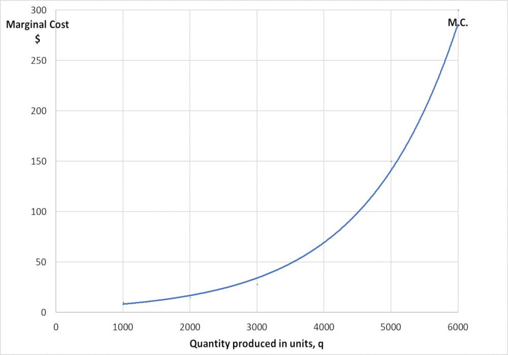 As quantity produced increases the M.C. is steeper.
Profit maximization
From the graph below we conclude the M.C. curve is the supply curve in the short run in perfect competition we explain below. Please note that the average revenue(A.R.) curve (A.R. is the revenue that is earned by the producer on selling each unit of output. It is the total revenue divided by the total output. It is the price of the product.) and the marginal revenue(M.R.) curve (M.R. is the change in total revenue by selling one additional unit of output) are the same, parallel to the x-axis only in perfect competition(pc). The graph below is for all markets.
Figure 2
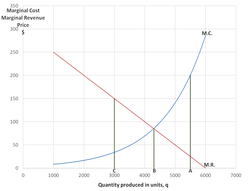 From figure 2 at output A, M.C. is more than the marginal revenue(M.R.) which in perfect competition is the price. M.C. is greater than the price. The firm loses money so it will produce less. At output C, M.R. is greater than M.C. the price of one unit of output is $150- the M.C.=$33-. The firm gains profit and it will produce more to gain more profit until M.C.=M.R. at B (see figure 2). If it produces more than B M.C.>M.R. the firm loses money. The firm will produce at B where Price=M.C. The firm produces where the price of the product=M.C. it produces that output. Therefore, the M.C. curve is the supply curve in perfect competition(pc). At a given price how much it will produce: supply curve.
In markets except pc: as output increases M.C. increases due to diminishing returns. At higher M.C. there is a higher M.R. curve to intersect it which leads to a higher A.R. curve(M.R. and A.R. are interrelated) which A.R. is the demand curve the price: Higher output higher price: figure5.2
In economic theory price is always determined by M.C. curve, M.R. curve and A.R. curve which is the demand curve.
Consider the following example of a pizza firm, in the year 2018, for simplicity values are rounded:
| Output production units of pizza per year |
Price per unit of pizza $ |
|---|---|
| 3,000 | 3 |
| 4,000 | 4 |
| 5,000 | 6 |
| 6,000 | 9 |
| 7,000 | 13 |
The accountant of the firm can provide the selling price for different values of output and will be like the table above. Recent past data with other values than the current value can be used, adjusted for inflation, to give the values in the table. By an interpolation(given the values the equation is derived) calculator these values give the function:
P= (q2)/2,000,000 -q/400 +6
P: price per unit of pizza
q: quantity in units of pizza
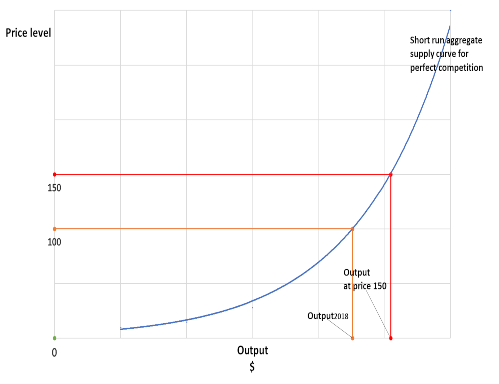
Now we take 2018 statistics, for example, the total production of units of pizza in 2018 of the economy is 100,000 and the price is $6- per unit. We take the 2018 prices to be price= 100-. Now if price increases by 50% the new price= 150-. This means that now the price of pizza is $9- (6x1.50= 9). From the table above we find the corresponding output which is 6,000 units of pizza.
| price | output | Total production |
|---|---|---|
| 6 | 5,000 | 100,000 |
| 9 | 6,000 | x |
(6,000✕100,000)/5,000= 120,000- units of pizza
A better method: if price increases by 50% we find the new price: $9- and the corresponding output from the equation:
P= (q2)/2,000,000 -q/400 +6 from an inverse function calculator we find: Output=q=500(√ 8P-23 +5)
Output=q=500(√ 8✕9-23 +5)= 120,000- units of pizza
assuming that the market share of pizzas of the firm in the example remains the same and also the supply curve of the pizza firm is the same shape with the other pizza firms which are both acceptable assumptions to make. We do the same with all other goods and services in GDP(national output or national income(Y)) we choose one representative firm and calculate the total production of the industry as it was with pizzas and add them all up.
Then we find:
| Price | N.Y.(Y) |
|---|---|
| 100 | GDP2018 |
| 150 | (6*✕120,000(no. of pizzas) +all other...) |
We plot a graph by finding the points:
(100, GDP2018)
(150, as calculated)
(200, calculated)
Perfect competition
Using the above technique we apply it to perfect competition(pc) and we derive the pc equation and graph by interpolation:
P=αY n+βY n-1+...+γ
αY n+βY n-1+...+γ>0, n integer >0, dP/dY>0, d2P/dY2>0
Figure 3
Monopoly
In monopoly, there is no unique relation between market price and quantity supplied. There is no distinct supply curve under monopoly. Yet when the demand curve shifts to the right (increases) there is a relation between increase in prices and increase in quantity supplied as the following graph shows under the assumption that the demand curve shifts parallel:
Figure 4
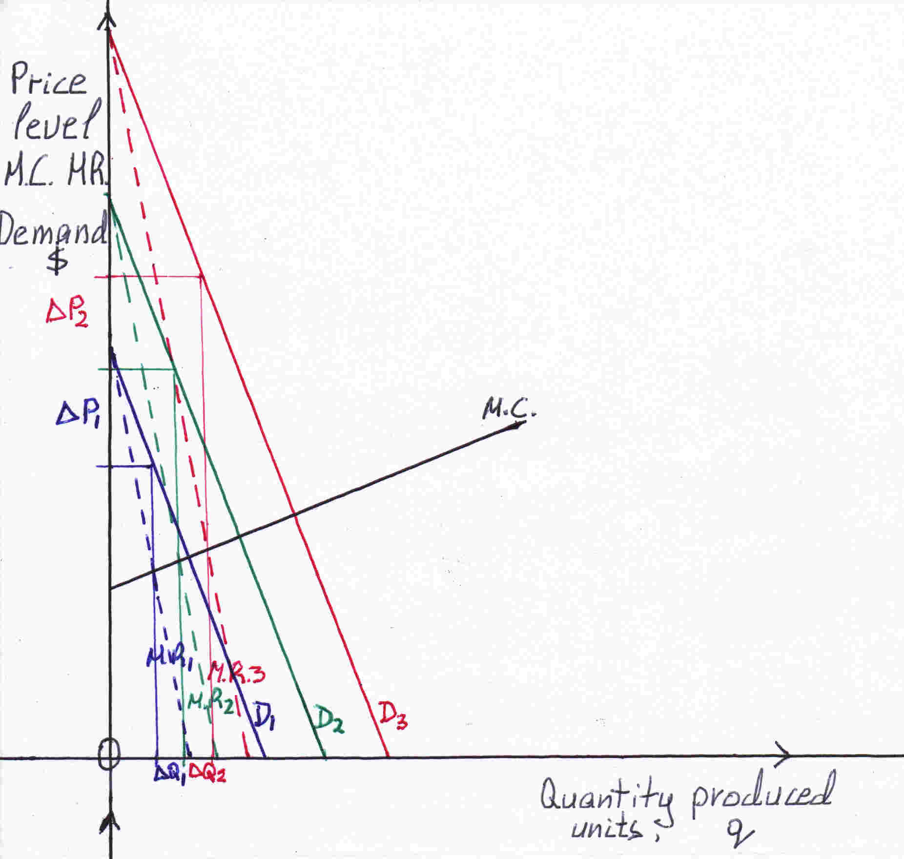 The monopolist produces that output where M.C.=M.R. to maximize profit as it was explained. From the graph above you can see the output determined is at the intersection of the M.C. curve (black line-) and the M.R.1, M.R.2, M.R.3 curves (dotted lines). The monopolist sets the price at which consumers are willing to pay at the determined output the demand curves D1, D2, D3. Where the output meets the demand curve we get the price. From the above graph you can see that the change in quantity ΔQ increase is less than the change in price ΔP (increase). The price compared to quantity increases at a larger rate.
Please see figure 5, below.
The demand curve is the average revenue(A.R.) curve:
A.R.=Total revenue/quantity = price✕quantity/quantity = Pq/q = P
Let the equation of the demand curve be PD=mq+c where m: slope, c: intersection to the y-axis or Price-axis
Marginal Revenue= d(T.R.)/dq = d(PDq)/dq = d(mq2 + cq)/dq = 2mq+c
The slope of the demand curve is m and is negative. As proved the slope of the M.R. curve is 2m it is twice as steep.
The A.R. curve meets the q axis:
0=mq+c
mq=-c =>q=-c/m
The M.R. curve meets the q-axis:
0=2mq+c =>q=-c/2m
The horizontal distance from(0,0) is half for the marginal curve. When M.R. is zero it intersects the q-axis at q=-c/2m at that q the A.R.= mq+c= m(-c/2m) + c= c/2
When M.R.=0 A.R.= c/2
A.R.=y
M.R.=x
M.C.=z
mc: slope of the M.C. curve
cc: intersection of the M.C. curve to the y-axis or Price-axis
x1=2mq1+c1
x2=2mq2+c2 => Δx= 2mΔq+ Δc
At the two points of intersection between M.R.s and M.C. we have:
z1=mcq1+cc
z2=mcq2+cc => Δz= mcΔq
∴Δz= Δx
∴mcΔq= 2mΔq+ Δc
∴Δc= mcΔq- 2mΔq —✱
y2= mq2+ c2
∴Δy= mΔq+ Δc
From just the above equation and from ✱: Δy= mΔq+ mcΔq- 2mΔq
∴Δy=mcΔq- mΔq
∴Δy= (mc -m)Δq
∴ΔP= (mc -m)Δq
∴ΔP/Δq= mc -m
∴P= (mc -m)q+ γ2
∴P= β2q+ γ2
β2= mc- m, mc>0 the slope of the marginal cost curve, m<0 the slope of the demand curve which is negative so -m is positive therefore β2>0, γ2 is a number
Figure 5
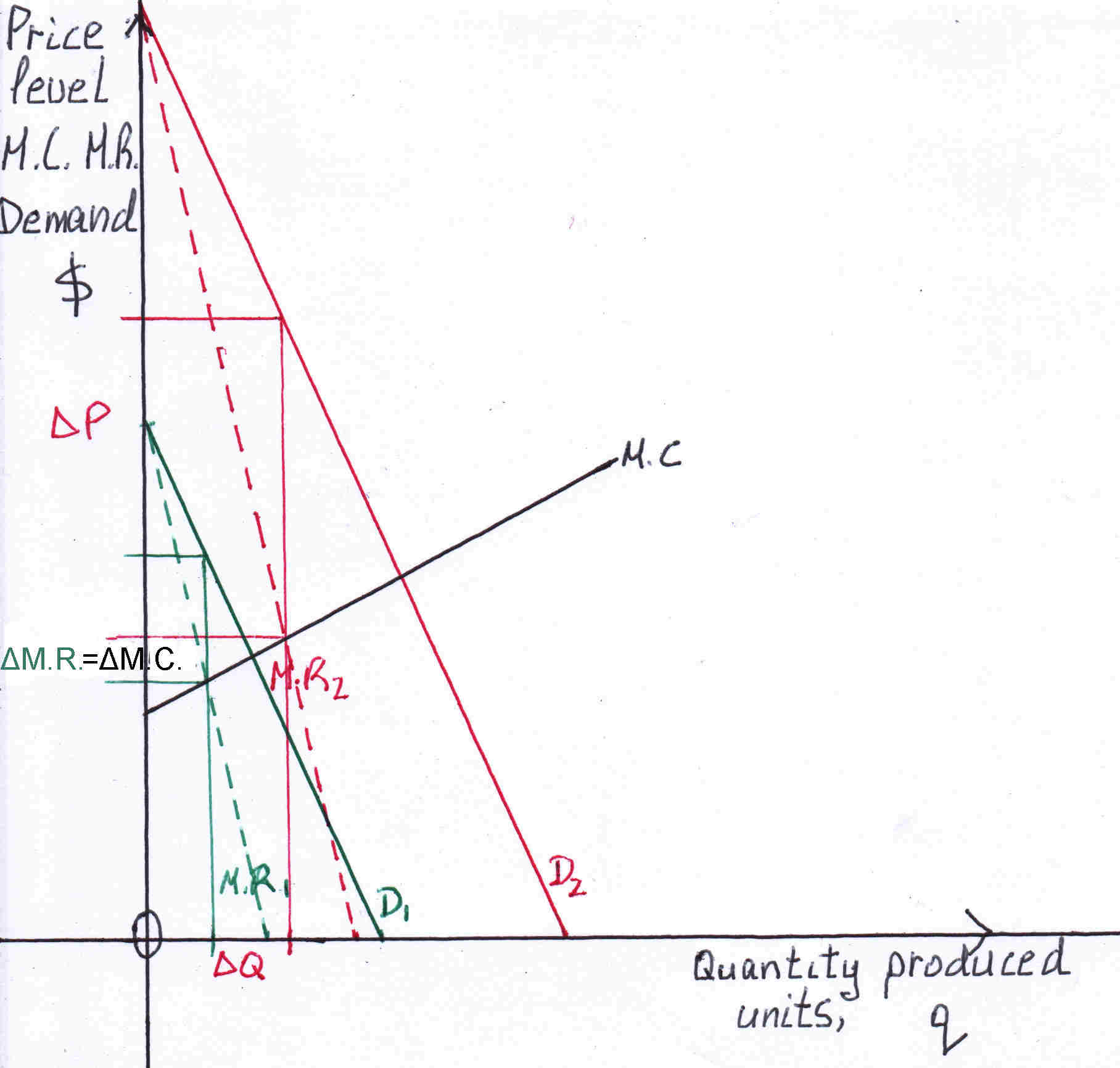 Why is the demand of a monopolist steep, |m| is high?
Because consumers cannot switch to another brand it is monopoly. A change in price brings a small change in quantity sold and thus produced. Therefore we relax on the assumptions that the demand curve shifts and not pivots(elasticity of demand changes dramatically) and also the M.C. is a straight line that does not shift (please see figure 5).
To express q units of output produced into Dollars we multiply q by price2018: output produced in Dollars. We multiply every value of q by price2018 as we did earlier in perfect competition.
We find β'2 and γ'2 by interpolation we know one point P=100, p2018q2018 output of the monopoly.
P= β'2pq+ γ'2
If the above monopoly(1) is 30% of the output of all monopolies then:
0.3P= 0.3β'2pq+ 0.3γ'2
∴0.3P= 0.3β'2Y(1)+ 0.3γ'2
∴0.3P= 0.3β'2✕0.3Ym+ 0.3γ'2
We add all other monopolies so Pm= β2Ym+ γ2
Therefore the point 2018 will be:
P=100, Ym(p(1)2018q(1)+p(2)2018q(2)+...)
p(1)2018 is the price of 2018 of monopoly(1)
q(1) is the 2018 output at price2018 of the monopoly(1)
Figure 5.1
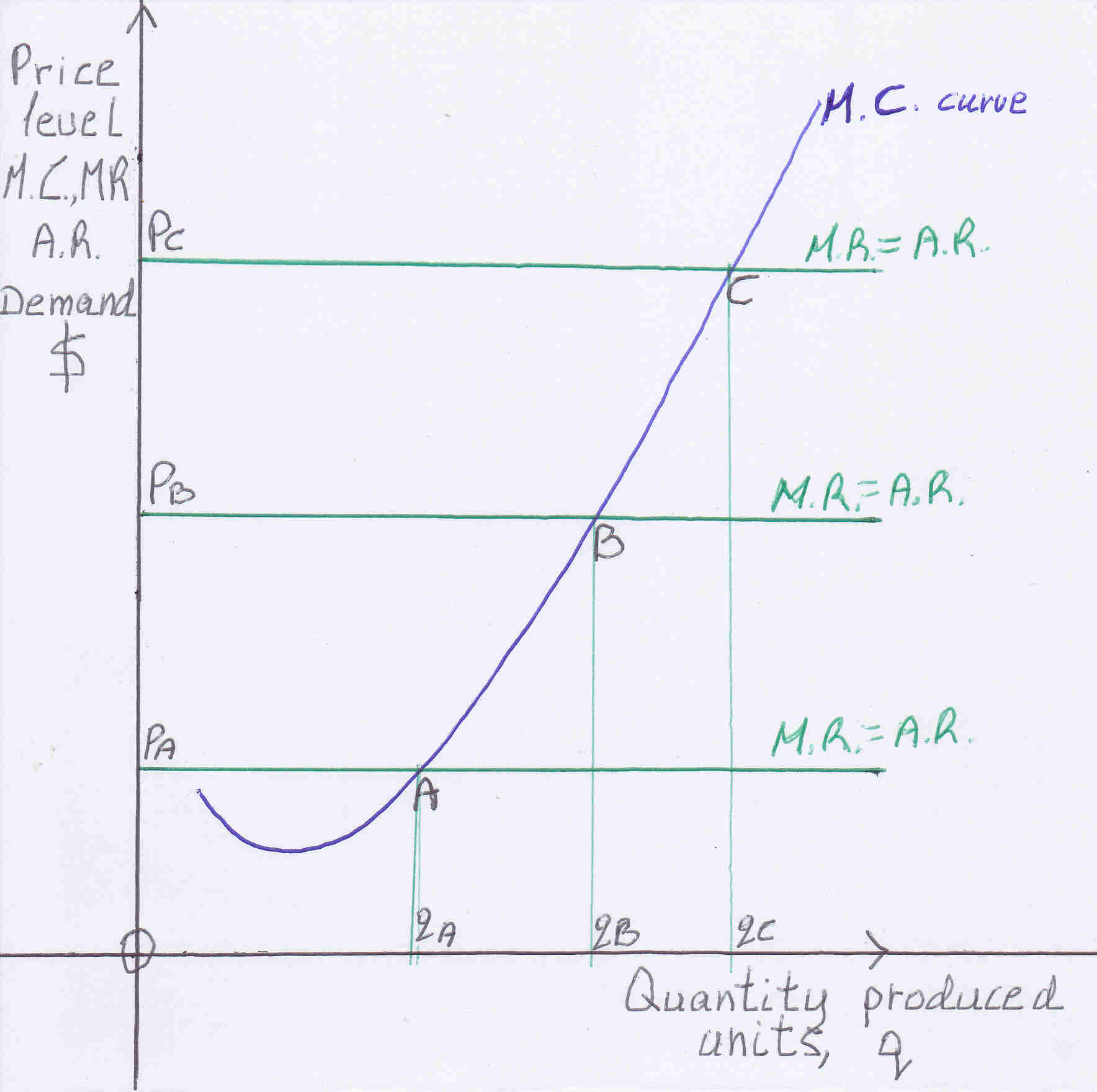 As explained previously the perfect competitive firm will produce that output where M.R.=M.C. to maximize profits. The M.R. curve is the same as the A.R. curve which is the demand curve and it is parallel to the x-axis and to other demand curves. The points of intersection between M.R. curves and the M.C. curve describe the supply curve for example at PA it will produce qA, at PB it will produce qB, at PC it will produce qC but these points as it is illustrated is the M.C. curve: points A, B, C.
Figure 5.2
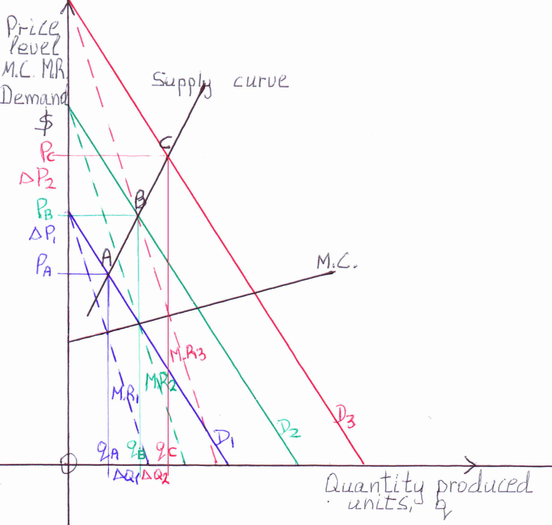 Please, see also figure 4. In monopoly the monopolistic firm will produce the output where M.R.=M.C. to maximize profits where M.C. curve intersects the M.R. curve. At that output we find the price we move upwards vertically until we meet the demand curve, D, of the monopolistic firm. There, is the price of the product. Therefore, at output qA the price is PA. At output qB the price is PB and at output qC the price is PC. The line which connects these points A, B, C,: (qA, PA) (qB, PB) (qC, PC) is the supply curve of the monopoly the philosophy is the same as in perfect competition. Of course, we assume that the demand curve shifts parallel to the previous demand curve. If it pivots we connect the points as done above and we will find the supply curve.
Monopolistic competition
In monopolistic competition there are many firms with freedom of entry and exit (competition). Yet each firm has some power over price because each sells a product that is somehow different from the firm's competitors (monopoly). The demand curve is rather elastic because there are substitute products from other firm competitors: As it was mentioned in monopoly the demand curve does not pivot because the elasticity of demand normally does not change it is a monopoly, consumers cannot switch to other goods. In monopolistic competition, however, the demand curve of a firm pivots because consumers can consume other similar products as the graph below demonstrates.
Figure 6
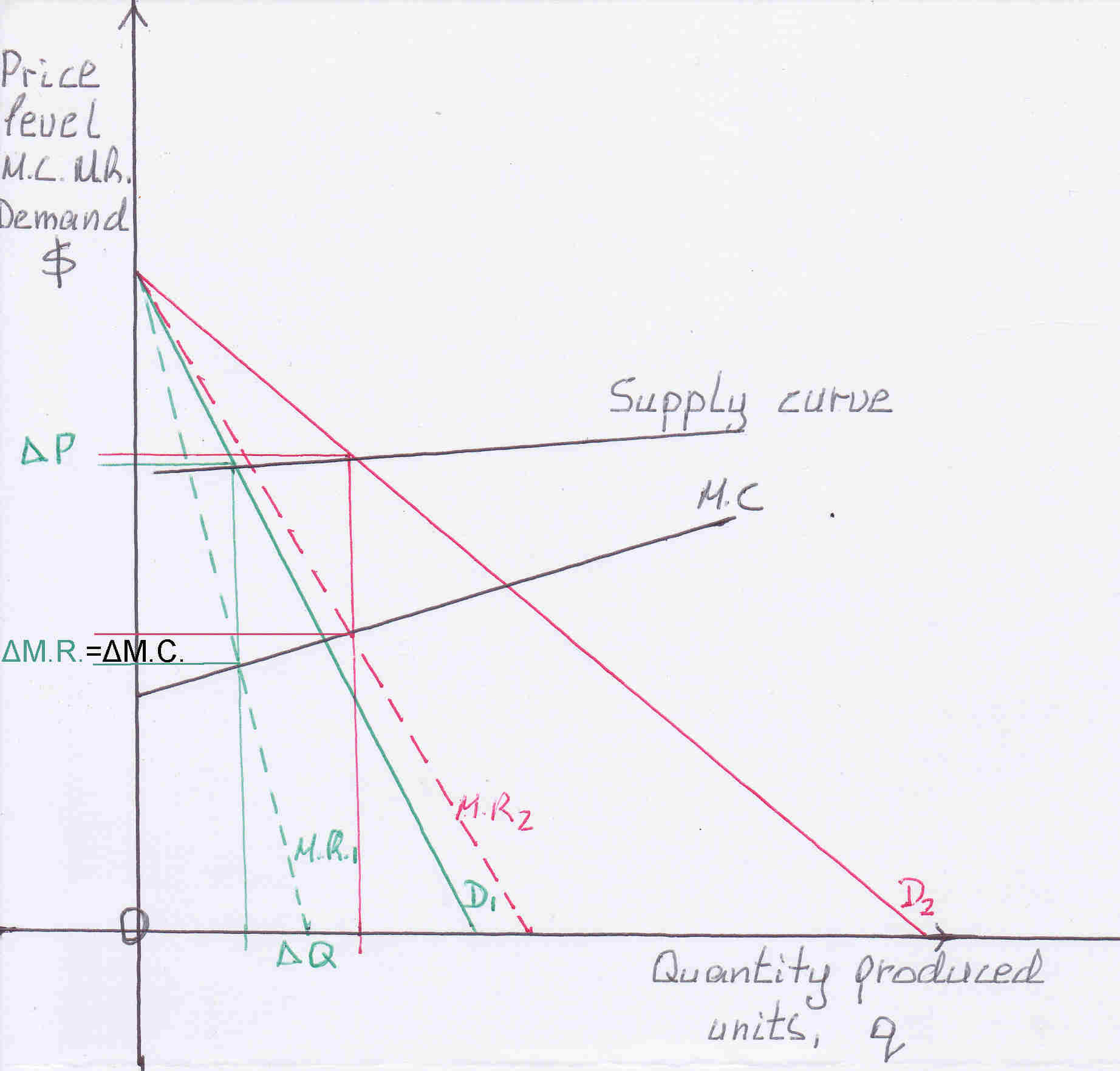 When the demand curve pivots from D1 to D2 there is a small change in price ΔP.
We showed in monopolistic competition(mc) that variation in quantity changes the price.
Now let:
A.R.=y
M.R.=x
M.C.=z
mc: slope of the M.C. curve
c: intersection of the A.R. & M.R. curves or y & x curves to the y-axis or Price-axis
cc: intersection of the M.C. curve or z curve to the y-axis or Price-axis
y1= m1q1 + c
y2= m2q2 + c
∴Δy= m1q1 - m2q2
x1=2m1q1+c
x2=2m2q2+c
∴Δx=2m1q1-2m2q2
z1=mcq1 + cc
z2=mcq2 + cc
∴Δz=mcΔq
But Δx=Δz
∴2m1q1 - 2m2q2= mcΔq —✱
But Δy= m1q1 - m2q2
From just the above equation and from ✱: Δy= 1/2mcΔq
∴y= 1/2mcq + γ'
P= 1/2mcq + γ'
Pmc(1)= β'Ymc(1)+ γ'
∴β'= 1/2mc, γ' is a number
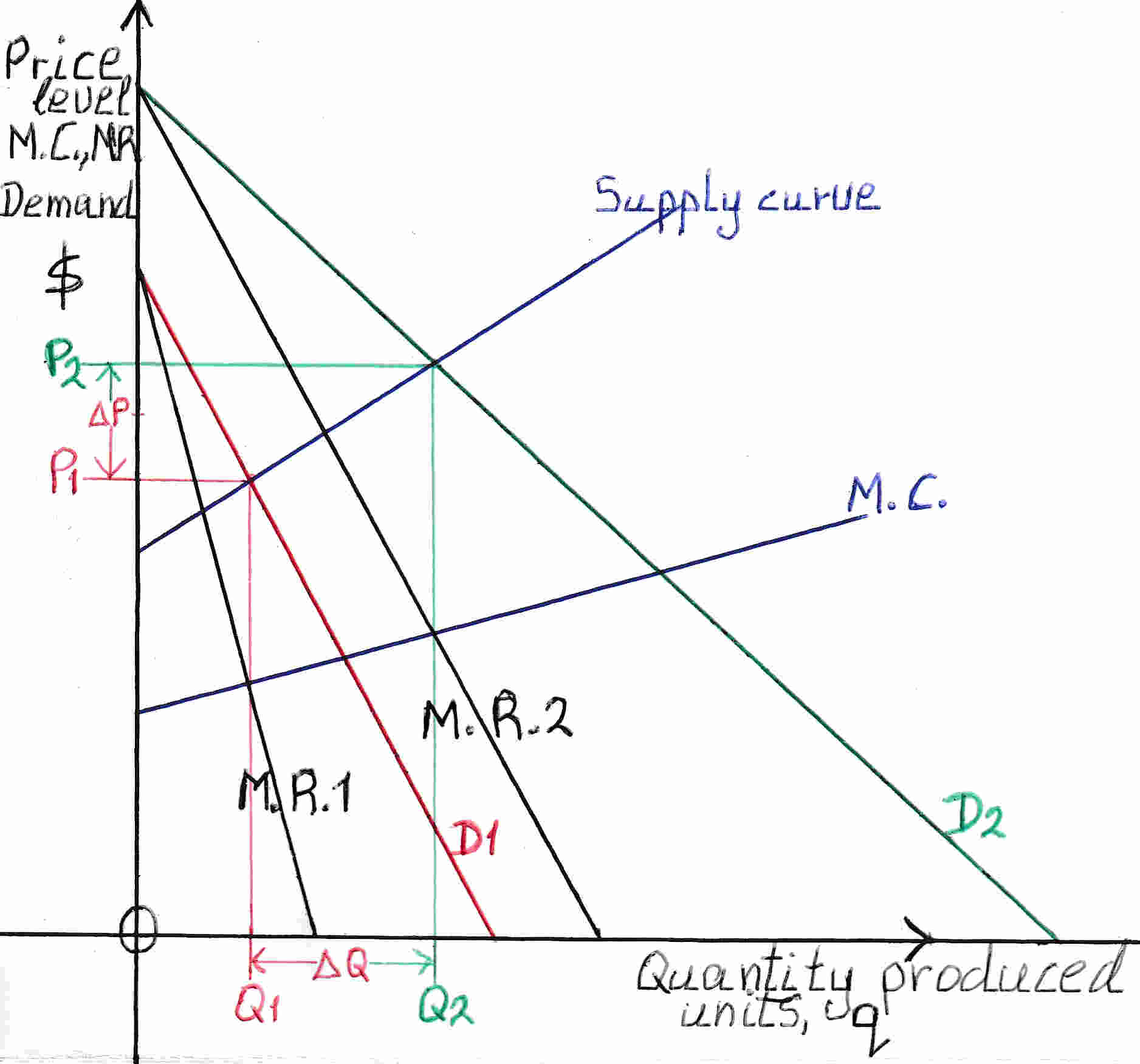 What if the demand curve moves randomly like in the graph above from D1 to D2:
Profit maximization is when M.R.=M.C.
Now let
Cc: intersection of the marginal cost curve to the y-axis.
C1: intersection of the initial demand curve D1 or A.R. curve and M.R. curve to the y-axis.
C2 intersection of the subsequent demand curve D2 or A.R. curve and M.R. curve to the y-axis.
mc: slope of the marginal cost curve.
m1: slope of the initial demand curve D1 or A.R. curve.
m2: slope of the subsequent demand curve D2 or A.R. curve.
Q1, P1: x, y at Point 1
Q2, P2: x, y at Point 2
We find Point 1
M.R.= M.C.
2m1q1 + C1 = mcq1 + Cc
2m1q1 - mcq1 = Cc - C1
Similarly we find Point 2
P = βY + γ, γ is a number
What if the demand curve moves randomly again? We find the Point 3 by equating M.R.=M.C. as done above. We, then, do either regression analysis (best line through the points) or interpolation (best equation that describes the points) and we find the best possible equation of Price and quantity. We know one point P=100, p2018q2018. We can take real, actual monopolies, all firms in monopolistic competition of a particular product and collusive oligopolies and observe the relationship between Price and quantity produced.
Subsequently, we do the same analysis as done in technical information 1 and monopoly, the principle is the same, and we derive the equation of the monopolistic competition:
Pmc= β3Ymc+ γ3, β3>0, γ3 is a number
Oligopoly
In oligopoly few firms compete with each other. Each firm has enough power so that it cannot be a price taker(take price as given), but it is subject to enough inter-firm rivalry that it cannot consider the market demand curve as its own. This is probably the dominant market structure outside agriculture and basic industrial materials. In oligopoly the price is sticky:
Figure 7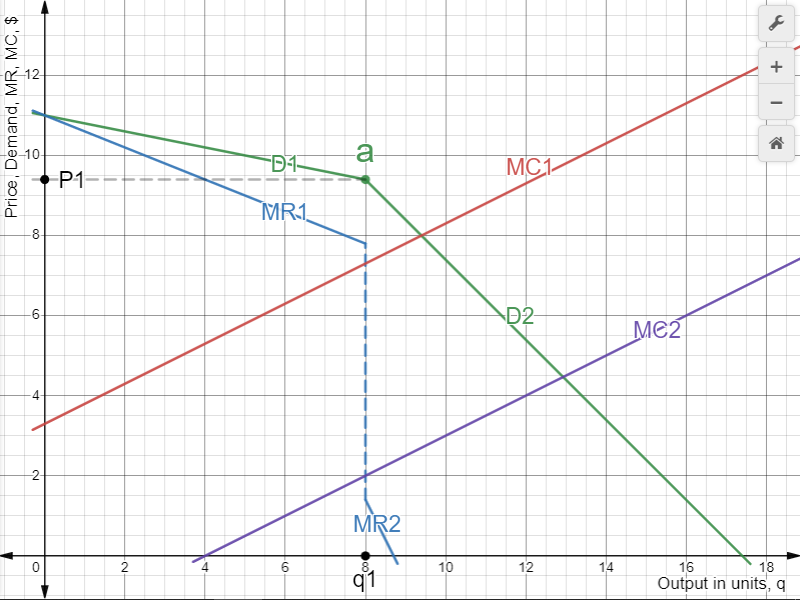
In the figure above the oligopolistic firm is assumed to be selling q1 units at a price of p1. It then considers altering its price and it makes two key assumptions. First, it assumes that if it cuts its price, all of its competitors will match its price cut. Its demand will then expand along the relatively steep curve below a, which indicates the effect of the firm's price cut when its share of the market is unchanged. Second, it assumes that if it raises its price, above p1, none of its competitors will raise theirs. Its demand for prices above p1 thus contracts along the relatively flat curve indicating the effects of raising prices with a declining market share. To summarize, above price p1 the competitors will not increase the price thus the firm loses a lot of demand: a small increase in price leads to a large decrease in demand the demand curve is flatter. At price below p1 the competitors will also reduce the price there will be no change in the firm's demand, competitors follow suit therefore the demand curve is steep a change in price brings a small change in output. Therefore, changes in the (M.C.) do not alter the price: see figure 7 M.C.1, M.C.2.
Figure 8
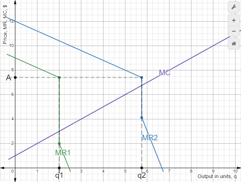 See the figure above: as demand increases the demand curve and thus the marginal revenue(MR) curve shifts from MR1 to MR2 the quantity changes from q1 to q2 but MR(point A) remains the same because price remains the same.
In oligopoly as quantity changes price is constant.
Po= 100
Adding up all markets
To conclude, we add up all markets of the economy as displayed above to derive the short run aggregate supply curve (s.r.a.s.c.) of the economy. We assume that perfect competition= 10% of the economy, oligopoly= 50%, monopoly=10% and monopolistic competition= 30%. Therefore, Ypc= 0.1Y=> Ypcn= 0.1nYn and Ym= 0.1Y. The Ppc to express it in terms of Price, P for the whole economy we multiply the whole pc equation by 0.1 because this is the share of pc in the economy to derive the weighted average for the whole economy (Ppc=0.1P). We integrate the analysis done separately before and the just previous assumptions and we have:
Perfect competition
0.1P= 0.1α1✕0.1nY n+...+0.1✕0.1β1Y+0.1γ1
Monopoly
0.1P= 0.1✕0.1β2Y+ 0.1γ2
Monopolistic competition
0.3P= 0.3✕0.3β3Y+ 0.3γ3
0.5P= 50
The above equation applies for Y≥Yavc.min because the supply curve for pc is at an output, Y, greater or equal than where the minimum of the average variable cost(avc) curve occurs because at a value less than the minimum avc firms make losses hence they close down, it will be later explained and proved in detail.
For Y<Yavc.min:Pc is not included that is 10% of the economy is not included the remaining is 90% to include the whole economy 100%: the increased share of the monopoly in the economy is: 100/90✕10%= 10/9✕0.1= 0.111= 11.111%:
Pm= 0.111β2Y+ γ2
0.111P= 0.111✕0.111β2Y+ 0.111γ2 —✱
Monopolistic competition 33.333%
Pmc= β3Ymc+ γ3
Pmc= 0.333β3Y+ γ3
0.333P= 0.333✕0.333β3Y+ 0.333γ3 —✱
0.556P= 55.556 —✱
Overall the s.r.a.s.c is a positively sloped curve which becomes steeper as national output increases because in the short run firms have a specified capacity leading to a s.r.a.s.c. which has a vertical asymptote at a large national output, please see figure 3.
An example with figures
Below there is an example of a s.r.a.s.c.:
The given equations are not the real US GDP they are just an example which resemble reality more realistic equations can be obtained from empirical evidence that is at given prices how much the producers are willing to produce as explained before. The base year, Price=100, is 2018. US GDP2018= $20.5 trillion.
Perfect competition
The equation for perfect competition(pc):
Ppc= 176Ypc4-859Ypc3+1571Ypc2-1279Ypc+411.878
Please, note that the supply curve for pc starts where the M.C. meets the Average Variable Cost curve (a.v.c.c.) at minimum. We have to derive the a.v.c.c. We integrate M.C. equation which is above and we get:
T.V.C.= 35.2Ytvc5 -214.75Ytvc4 +523.6667Ytvc3 -639.5Ytvc2 +411.878Ytvc +k
In the above equation T.V.C. is the Total Variable Cost(tvc), Ytvc is the output is the variable and k is a constant number.
The input of variable cost, for example, labor when it is 0 total variable cost is 0 and output Y is 0. Consequently, when Y=0, T.V.C.=0 substituting these values in the above equation we have:
k=0
∴T.V.C.= 35.2Ytvc5 -214.75Ytvc4 +523.6667Ytvc3 -639.5Ytvc2 +411.878Ytvc
Then we divide by Y because the above equation is the Total Variable Cost to derive Average Variable Cost:
A.V.C.= 35.2Yavc4 -214.75Yavc3 +523.6667Yavc2 -639.5Yavc +411.878
The a.v.c.c. is as in the graph below (red curve). We find the point of intersection of the two curves and indeed is the minimum of a.v.c.c. where the supply curve for pc starts: it is output=1.9704.
Now, because Ypc= 0.1Y, Y= Ypc/0.1= 10Ypc, Y=19.704 from that point pc equation is taken into consideration in deriving the s.r.a.s.c. Of course we later multiply by 0.1 but the a.v.c.c. is also affected, its minimum is the same: 19.704.
According to the above two equations: M.C. and A.V.C. the graph is as follows:
Figure 8.1
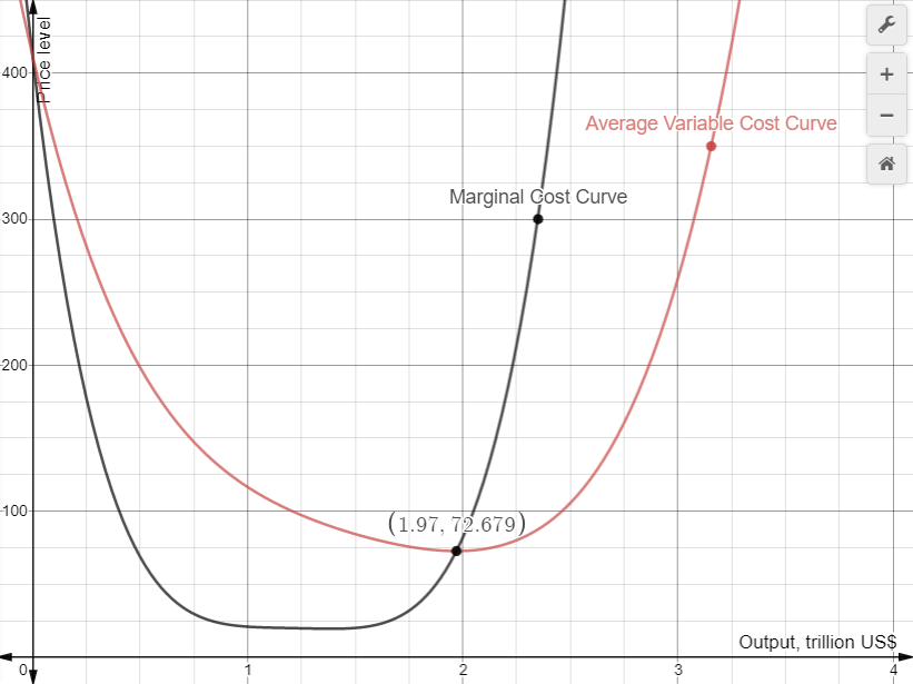 Now, as explained before Ypc=0.1Y we substitute 0.1Y for Ypc to express the above equation in terms of Y, national output:
Ppc= 0.0176Y4-0.859Y3+15.71Y2-127.9Y +411.878
The above Ppc to express it in terms of Price, P for the whole economy we multiply the above equation by 0.1 because this is the share of pc in the economy to derive the weighted average for the whole economy:
0.1P= 0.00176Y4-0.0859Y3+1.571Y2-12.79Y+41.1878 —✱
Monopoly
Pm= 2.1Ym +95.695
Pm= 0.21Y +95.695
0.1P= 0.021Y + 9.5695 —✱
Monopolistic competition
Pmc= 1.1Ymc +93.235
Pmc= 0.33Y +93.235
0.3P= 0.099Y + 27.9705 —✱
Oligopoly
0.5P= 50 —✱
P= 0.00176Y4 - 0.0859Y3 + 1.571Y2 -12.67Y + 128.7278 for Y≥19.704
For Y<19.704:
Monopoly
Pm= 2.1Ym +95.695
Pc is not included that is 10% of the economy is not included the remaining is 90% to include the whole economy 100%: the increased share of the monopoly in the economy is: 100/90✕10%= 10/9✕0.1= 0.1:
Pm= 0.23Y +95.695
0.1P= 0.0259Y +10.6327 —✱
With the same thinking:
Monopolistic competition
Pmc= 1.1Ymc +93.235
Pmc= 0.36Y +93.235
0.3P= 0.12Y +31.0783 —✱
Oligopoly
0.5P= 55.5 —✱
P= 0.148Y +97.267 (these numbers are rounded to three decimal places)
Combining the equations for Y≥19.704 and Y<19.704 the graph is as follows:
Figure 8.2
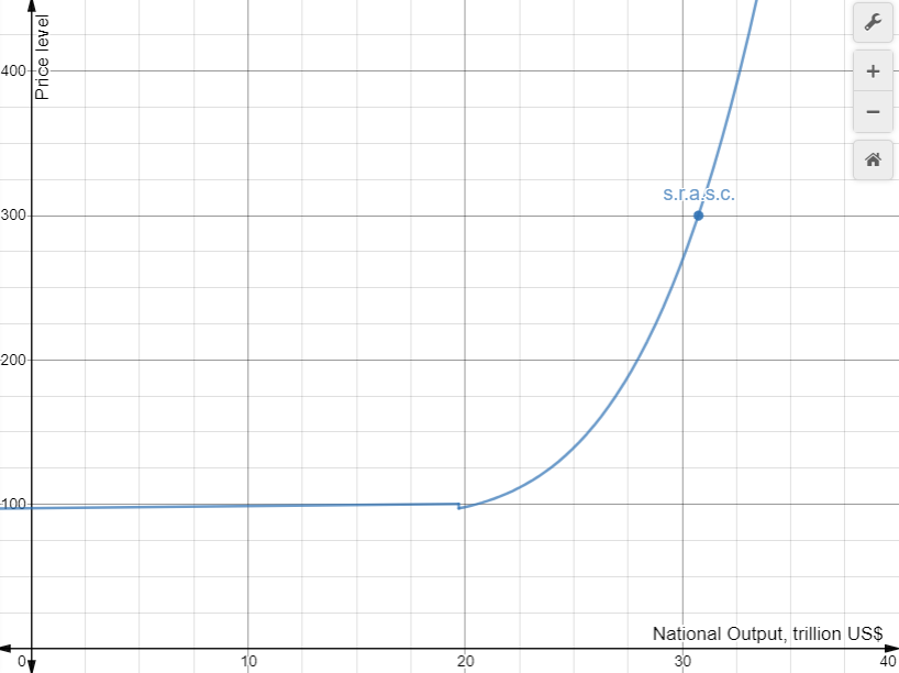 Since the two curves end and begin above each other we connect them with a vertical line to make them one curve. At Y=19.704 pc is included and Price drops slightly because goods and services in pc have lower Price than Monopoly, Monopolistic Competition and Oligopoly at Y<19.704 please see equations.
When A.D. increases
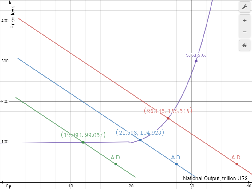
Please, see the graph below.
When aggregate demand, A.D. increases: shifts to the right, the increase in price is enough at low values of output. For example, in the graph from A.D.green to A.D.blue the price went from 99 to 105: change 6. Then by the same amount of increase in A.D. from A.D.blue to A.D.red the price went from 105 to 159: 54. This is because the supply curve as output increases becomes steeper. At full employment output (supply curve is vertical) an increase in A.D. causes high inflation and zero economic growth(annual percentage increase of real National Output, Y). The shift of A.D.green to A.D.blue Y increased (in trillions) from 12 to 22: 9. From A.D.blue to A.D.red Y increased from 22 to 26: 4. The above paragraph is merely an example to demonstrate the effects of changes in A.D. This is what is happening to the US economy right now: inflation is increased, economic growth is reduced.
Figure 9
When marginal cost changes
Figure 9.1
Shape of the s.r.a.s.c.
As output increases costs are rising at a faster pace. As output increases labor and raw materials become scarce so the wages, costs rise. Costs are also rising from diseconomies of scale and diminishing returns as previously explained. In all markets perfect competition, monopoly, monopolistic competition, oligopoly, the marginal cost curve leads to finding the output produced and the price (where the marginal cost(M.C.) curve intersects the marginal revenue curve: maximization of profit). For example, if the M.C. curve bends upwards: the equilibrium output q is restrained while the price increases. We are talking about one particular M.C. curve. Thus, as output increases the price increases at a faster pace giving us a short run aggregate supply curve which is upward sloping. At very high output the economy's potential is reached: full employment, full capacity, the M.C. curve becomes vertical, thus the output remains constant while price escalates.
To summarize:
As output increases costs are rising due to diminishing returns because costs are rising prices are rising as suppliers always maximize profit. Thus, in this instance as output increases price increases: upward sloping short run aggregate supply curve
From price's perspective:
As price increases producers increase output because at a lower price the increased output makes a loss.
Long run aggregate supply curve is vertical
The assumption in deriving the s.r.a.s.c. is that the factory buildings, heavy equipment remain the same. In the long run factory buildings, machinery increase. Thus the s.r.a.s.c. shifts to the right:
Figure 10
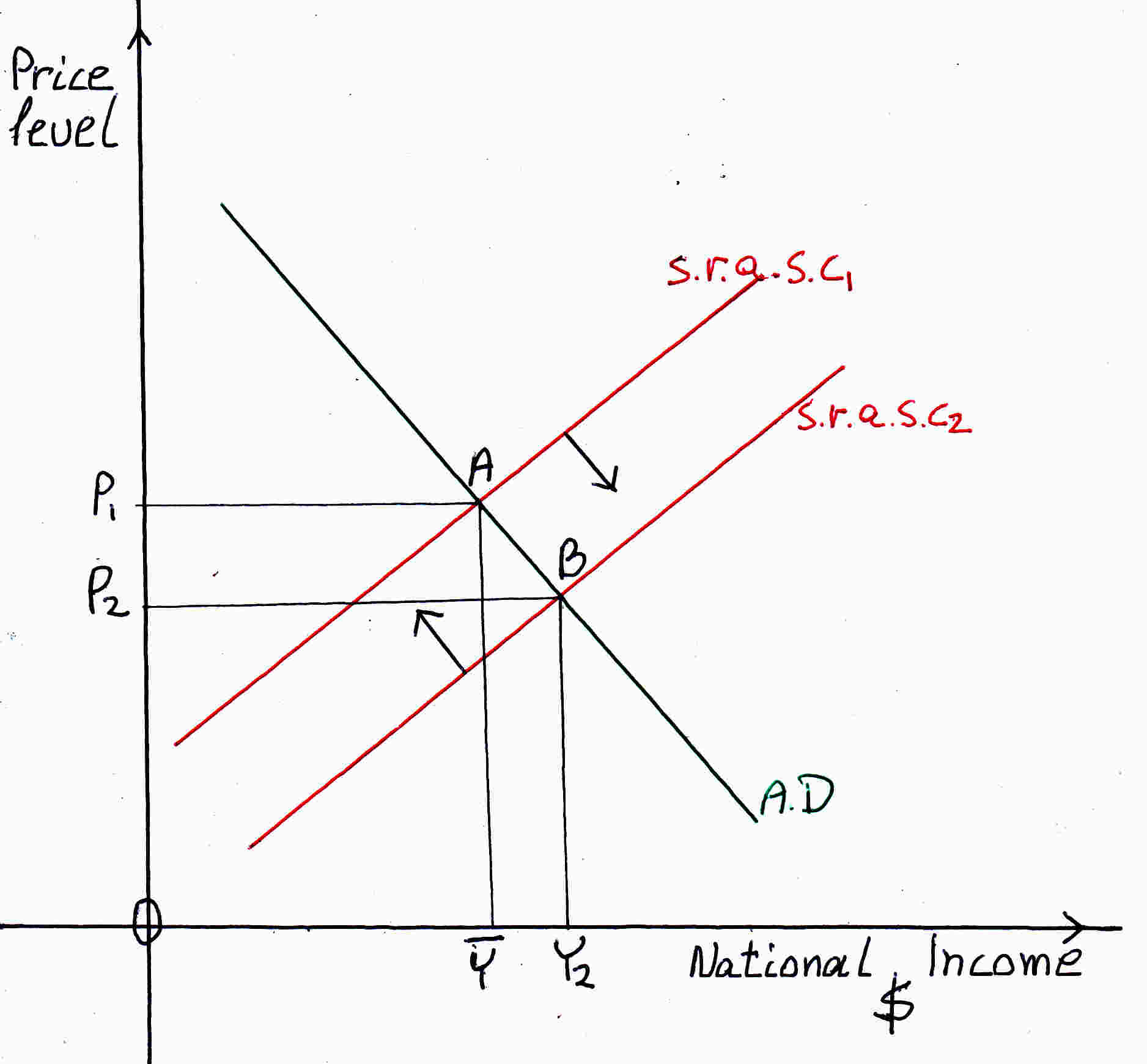 At equilibrium the economy is at its natural level of output (potential output) Y and the s.r.a.s.c. meets aggregate demand curve at point A. When buildings, machinery increase the s.r.a.s.c. shifts to the right s.r.a.s.c.2. At point B the actual output Y2 exceeds the potential output workers are scarce thus wages rise and s.r.a.s.c. shifts to the left to s.r.a.s.c.1. Therefore, at point A after the shift we have more factories and machinery and higher wages. In reality the economy is dynamic: aggregate demand and aggregate supply are ever-changing. The above example (figure 10) is a simplification, it demonstrates that the long run aggregate supply curve is vertical.
Liquidity trap
Figure 11
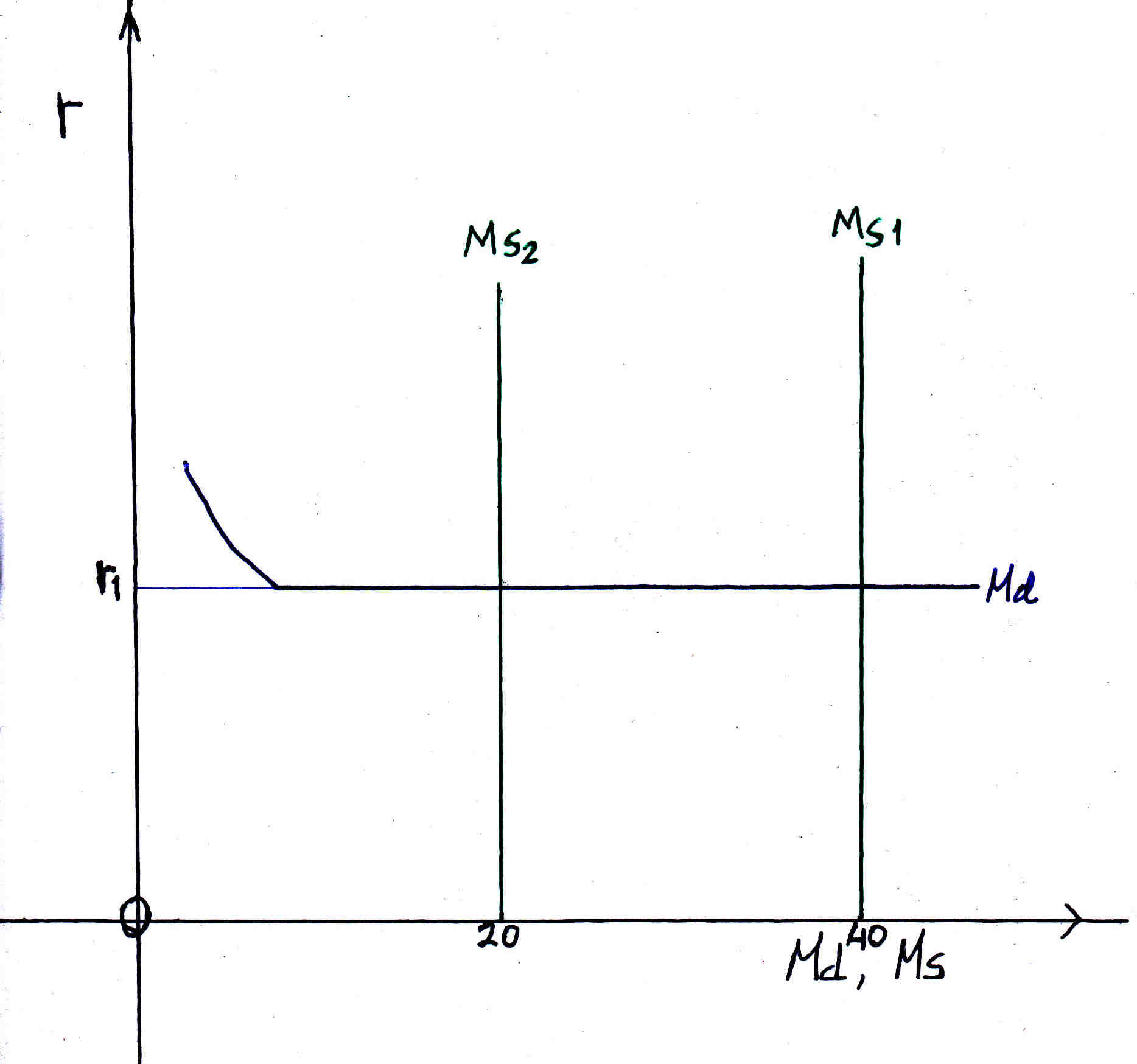 At liquidity trap the money demand curve (Md) is flat as money demand changes the rate of interest is the same r1. The money supply curve MS does not change with interest rate changes in fact the rate of interest does not have an effect on money supply it remains the same: 40. Suppose we have an increase in prices the real money supply decreases because real money supply= M/P= 40 where P is the price. If prices double then real money supply= M/2P= 20.
A change in prices does not change real money demand because the higher the prices the more money people will demand canceling each other out. Money demand= (M/P)d after doubling the price: (2M/2P)d= (M/p)d real money demand is the same.
From the previous graph the rate of interest is constant thus the LM curve is flat. Therefore, national income does not change it remains the same Y1 as in the graph below.
Figure 12
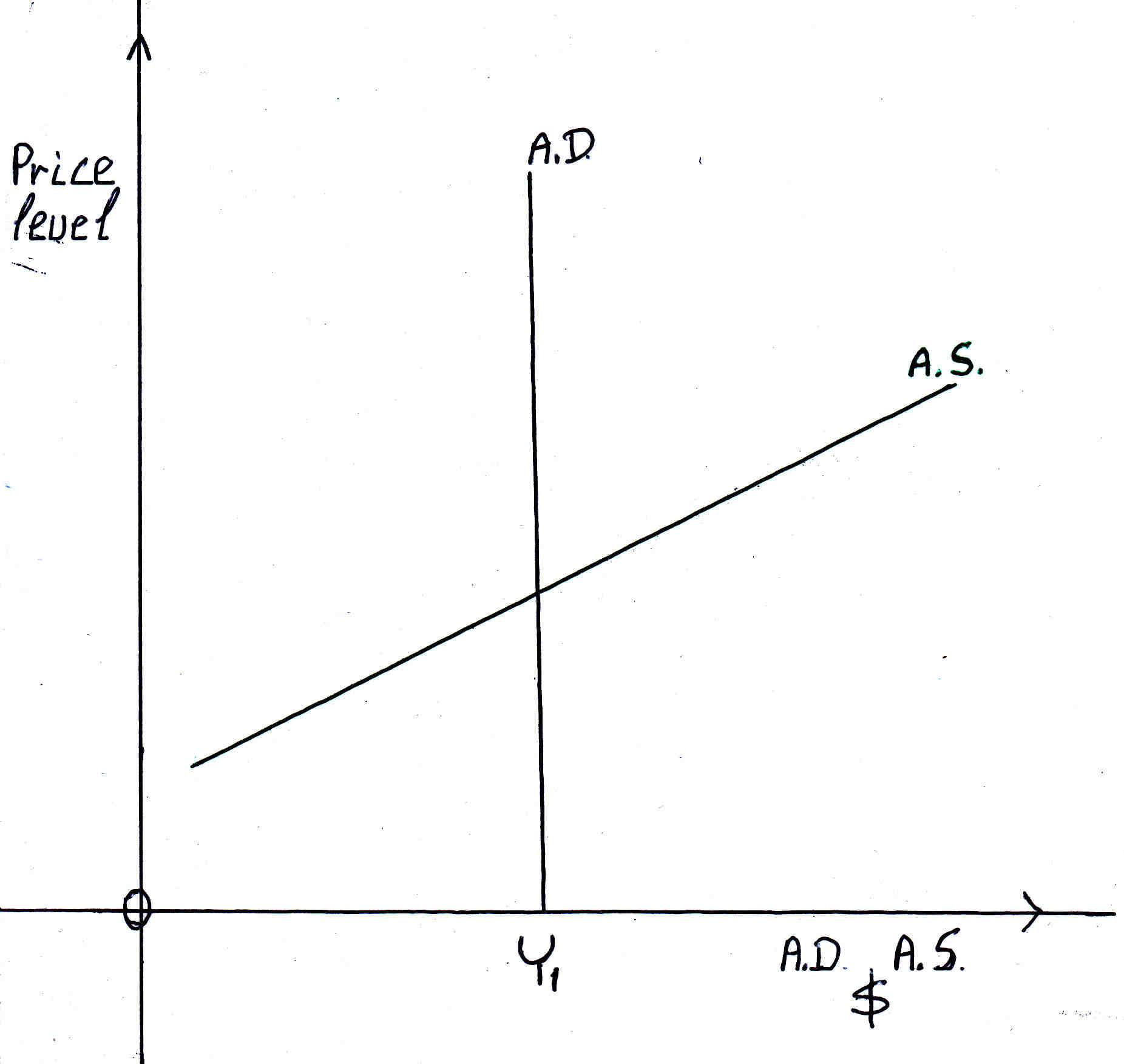
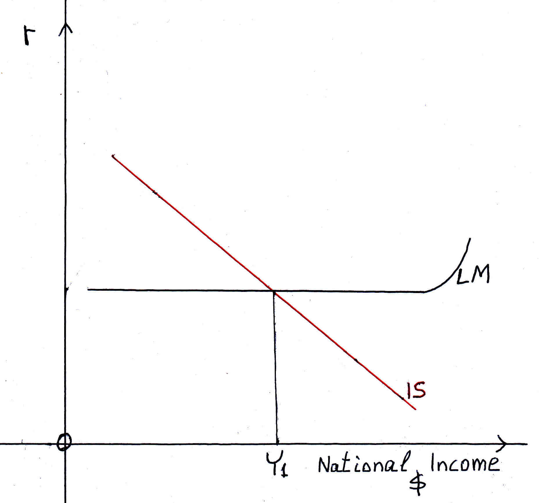 Because the Y1 remains the same we have a vertical national income or aggregate demand curve. As price changes A.D. is the same:
Figure 13
Average variable cost ≤ price, for production
In the short run a firm should produce if and only if total revenue is equal or greater than total variable cost. A firm to make a profit its total revenues must be greater than its total costs: T.R.>T.C. Profit= total revenues- total costs
Total costs= Fixed costs + total variable costs
Fixed costs: interest, rent, depreciation
Total Variable costs: labor, raw materials for the product
The fixed costs are there even if the output is zero the fixed costs exist.
In the short run the firm produces if the total revenues are equal or greater than the total variable costs. Why? Even if: total revenues- total variable costs= $1- the firm subtracts this one dollar from the fixed costs. The fixed costs will be $1- less. The fixed costs always exist. Except when the firm closes down.
Therefore the firm to reduce its fixed costs produces where the total revenue is equal to or greater than the total variable cost. At that point Total revenues= Total variable costs and at values where the total revenues are greater the firm produces and at that point onwards the marginal cost curve is the supply curve in perfect competition. Please bear in mind that
total revenues= price✕quantity produced
total variable costs= average variable cost✕quantity produced
total revenues= total variable costs
Therefore price✕quantity produced= average variable cost✕quantity produced
Therefore price= average variable cost(A.V.C.)
Consequently, in the short run, the firm produces where the price= average variable cost or at a greater price. This applies to all the markets in the economy: perfect competition, monopoly, monopolistic competition, oligopoly.
Figure 14
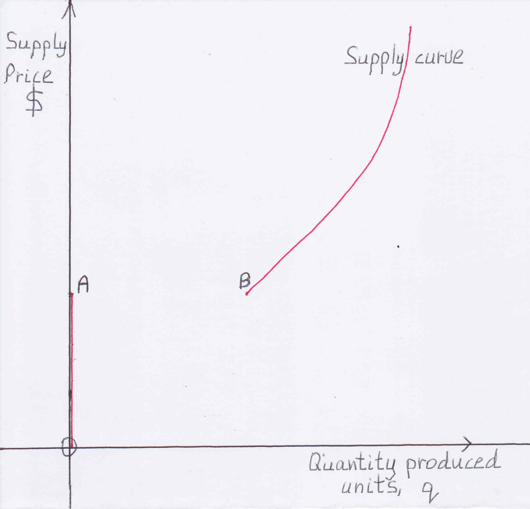 As it was previously explained the supply curve is the red line-curve (please see figure above). At price-output less than point B (less than A.V.C.) the firms close down. The supply curve is a vertical line along the vertical-axis, price-axis at output 0 until point A. Then the supply curve is the curve from point B onwards.
Figure 15
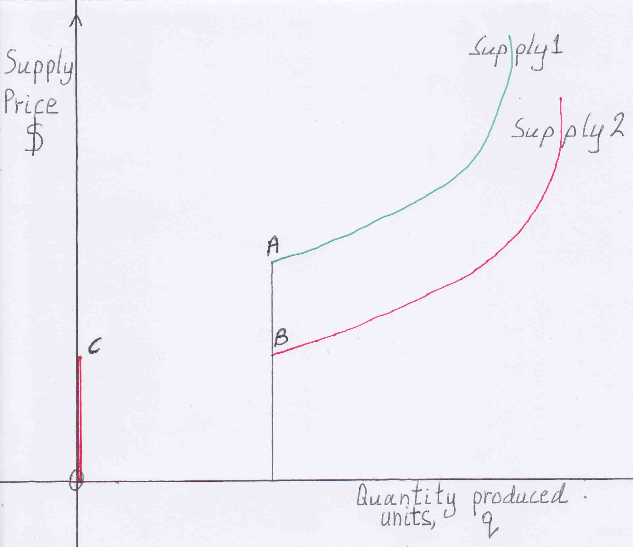 When wages, costs, prices fall: Supply curve shifts to the right, down (please, see the figure above). There is a vertical movement from A to B the supply curve moves vertically down from A to B the new supply curve is the red line curve. Please, note that at price less than B the supply curve moves from B to C. There is a horizontal movement from B to C.
When s.r.a.s.c. does not meet A.D.
Figure 16
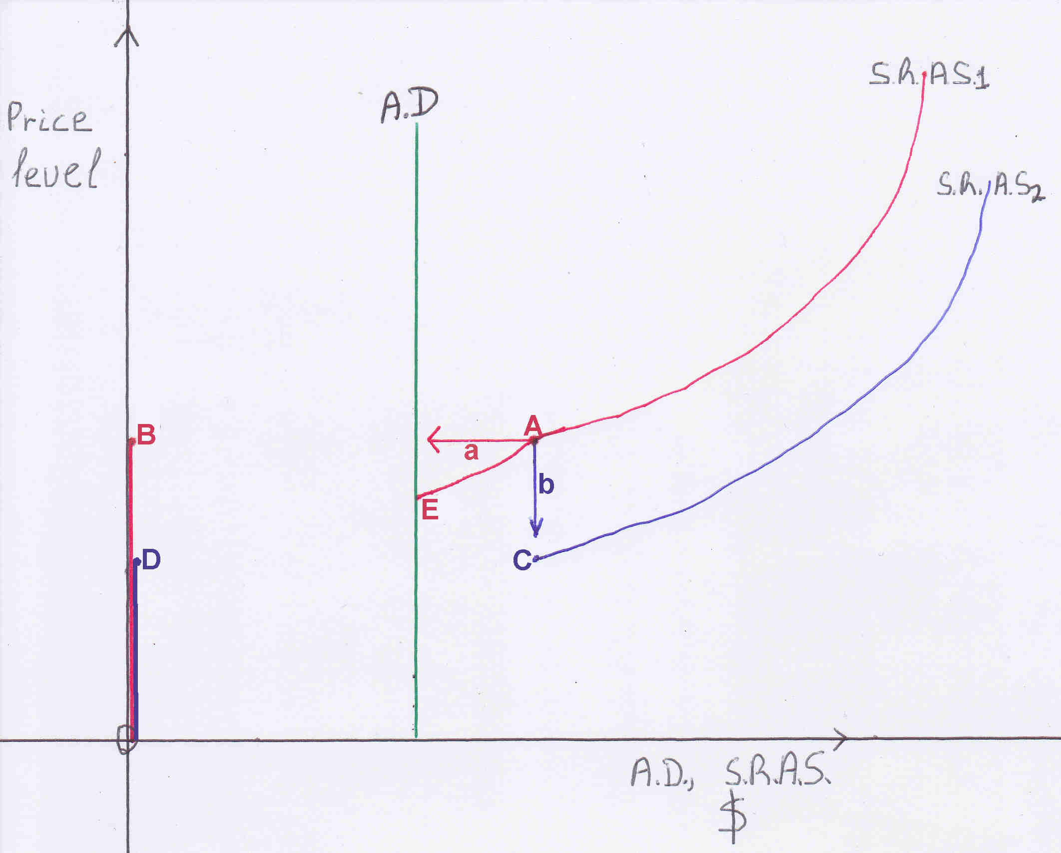
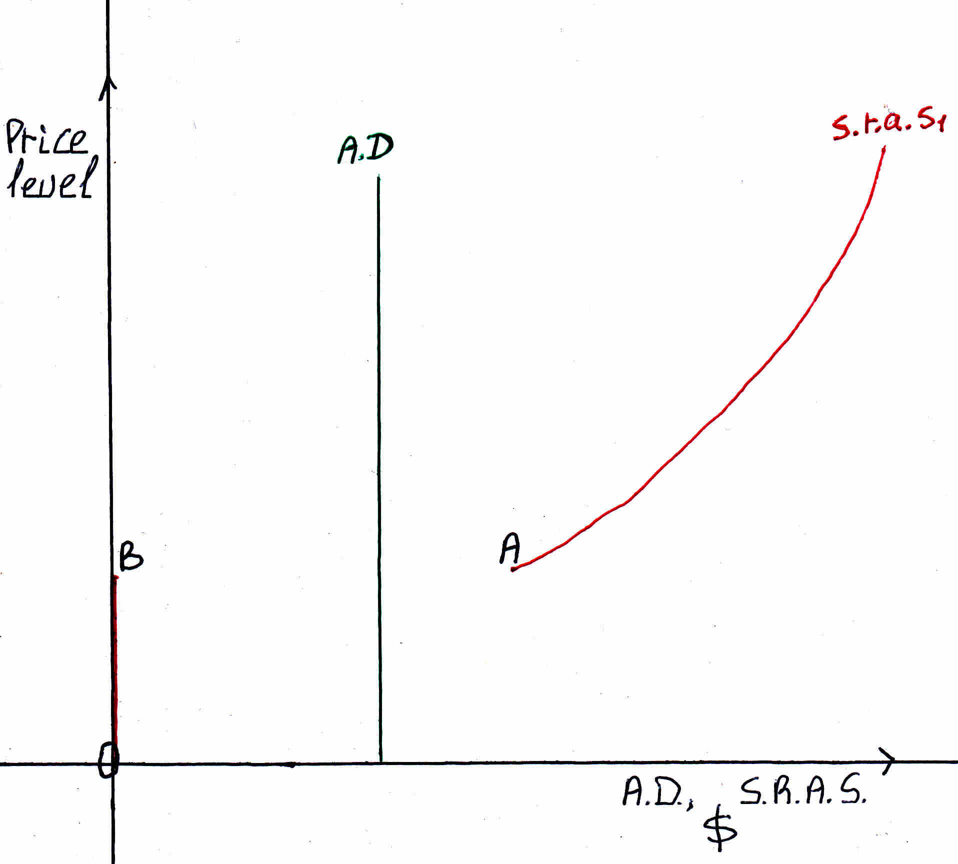 At the above graph there is inconsistency: point A the s.r.a.s.c. does not meet the A.D. curve. There is excess supply. When there is excess supply the prices fall. When prices fall below A the supply curve moves from point A to point B. What that means is that supply moves to zero, firms not having at least their average variable costs covered stop production they are closing down there is a movement: a arrow (please, see figure below). When firms are closing down unemployment increases demand for raw materials decrease. Wages and prices decrease therefore the supply curve falls there is a movement: b arrow. The result is a diagonal movement of the s.r.a.s.c. from point A to point E. At point E prices fell and output fell. This is what happened during the Great Depression in U.S.A. and to a lesser effect in Germany and Japan in 2009.
Figure 17
Liquidity trap
The problem with liquidity trap is that individuals do not deposit their money in the banks. The European Central Bank (ECB) injects money into the economy individuals take the money out of the economy by holding money as cash, money demand is flat please figure 11. Why is this happening? Europeans do not feel safe by depositing their money in the banks because the banks may default. What the ECB, Bank of England and Bank of Japan should do is to guarantee all bank deposits: in case a bank goes bankrupt the central bank will pay for the deposits and be legally bound to keep their word. Central banks have an unlimited supply of money. Secondly, even if all bank deposits are guaranteed individuals are indifferent of depositing their money because the rate of interest is very low. They do not forego any interest so they keep money as cash. Therefore, the interest rates should be increased this can be achieved by increasing the discount rate (the interest rate central banks charge the commercial banks for lending the commercial banks) and by increasing the funds rate (the interest rate banks charge each other). When banks need money they will sell bonds that they hold they will not borrow from the central bank or other banks because the rate of interest is higher. By selling bonds the price of bonds will go down the rate of interest will go up. There is the paradox how interest rates can increase (and they should be increased) and the economy and inflation grow? At a higher interest rate the opportunity cost of holding money increases individuals will deposit their cash injecting thus money into the economy. This will lead to banks using and/or lending money because they will have more cash from depositors and because the lending rate will increase. Banks will trade off between risk of loan and higher interest and they will lend more. I suggest the interest rate on deposits be driven to 3%. As US interest rate rose there is an upward pressure on the interest rates in the rest of the world. Do not fight these upward pressures let the interest rates rise. Thus, evading the liquidity trap. The above hold true for the Eurozone, United Kingdom and Japan. Also, with E.U. citizens leaving the U.K. there has to be a way of increasing the labor force. I think this could be achieved if a tax is imposed on couples who live in the same house and only one is working and they do not have child/ren below 6 years of age. The tax should be an additional tax of 10% on the income of the person who is working. If both people work this tax does not apply. The money received could be given to married couples who both work for example in the form of increased marriage allowance (allowance: a sum to be deducted from gross income in the calculation of taxable income). This is an incentive for people to work and be married. It will increase the British labour force participation rate. British housewives will displace E.U. citizens in U.K. The classic measure in eliminating liquidity trap is a generous fiscal policy please see figure 12 IS curve shifts to the right. It proved to work in USA but not in Japan which ran generous fiscal policies. Also, if the government wants to reduce the expenses to achieve budget surplus the generous fiscal policy measure cannot be used.
To my Japanese brothers
During the liquidity trap monetary policy is ineffective. Your government buys bonds keeping the wealth of households the same. Households give your government the bonds (decrease of wealth) and earn money (increase of wealth). Instead of owning bonds they own the same amount of money.
Fiscal policy which in liquidity trap is very effective your government sells bonds thus households receive the bonds and when the government spends the money from the sale of bonds households own the bonds and the money, their wealth increases.
National Income= GDP= C+I+G+NX
G is the government spending if the government spending increases the national income increases. It increases by the multiplier effect. Multiplier= 1/(1-mpc). Mpc is the marginal propensity to consume: how much of an additional 1 Yen is spent on consumption. By increasing G the GDP increases you have economic growth.
What can be done is a mixed monetary and fiscal policy: The Bank of Japan (BoJ) prints money or the government increases its deposits at the BoJ and increases the salaries of all Japanese people. It does not buy bonds which takes wealth (bonds) from Japanese households. By doing the above the national income will certainly grow by the amount of the (total increase of the salaries that is money printed) ✕ 1/(1-mpc). The interest rate remains the same, there is no crowding out. This measure will continue until inflation reaches an acceptable level. When you stop this measure the effect will go on for a period of time. The just above is demand-side economics, how A.D. is derived. How A.D. and A.S. interact please, see Figure 9.
Long run aggregate supply curve shifts
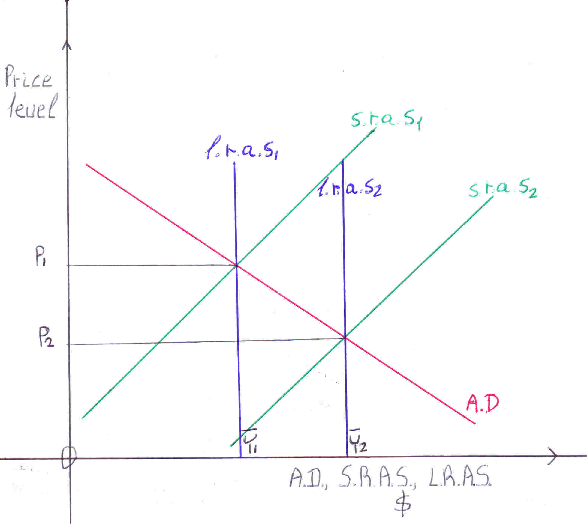
In conclusion, the s.r.a.s.c. is a diagonal curve starting from low price and low national output (Y) and as Y increases it becomes steeper, at large Y there is a vertical asymptote because in the short run firms have a maximum capacity and because of diminishing returns and diseconomies of scale. The s.r.a.s.c is derived empirically and perfect competition, monopoly, monopolistic competition and oligopoly are taken into account. Some effects of changes in A.D. are examined. In the long run the marginal cost curve shifts so the s.r.a.s.c shifts. Also, in the long run the s.r.a.s.c. shifts to the right because more buildings and machinery are used but the s.r.a.s.c. shifts back to the left because wages increase therefore the long run aggregate supply curve is vertical. At liquidity trap the A.D. is vertical and if it is low the s.r.a.s.c. does not intersect it leading to a reduction in both prices and Y. The short run supply curves hold true for price equal or greater than the average variable cost as previously thoroughly explained. Now, if s.r.a.s.c. shifts to the right and long run supply curve shifts to the right because natural level of output increases then prices fall and Y is increased, please see figure below. This can be achieved if the labor is increased if the number of workers increases. The US government can increase labor if it taxes couples living in the same house and only one is working and they do not have child/ren below 6 years of age by decreasing the tax deduction from their adjusted gross income. The US government can increase the tax deduction of couples who both work and are married with a church wedding and are husband and wife. This measure will increase the US labor force participation rate increasing the natural level of output Y decreasing the prices, please see figure below. How can productivity increase? The US government can introduce a measure that when an employer dismisses an employee the salary of the employee is deducted from the net profit before tax of the employer assuming no other person is then employed in a similar job of the dismissed employee. When a new employee takes the similar job this measure stops. This measure cannot be used if the period of the dismissal and employment is less than 3 months. This measure will reduce the number of unproductive employees and compel the employees to work more productively in order not to be dismissed. Also, it will have a positive effect on unemployment.
Figure 18
Tight fiscal policy
Is there a way to reduce inflation and simultaneously reduce interest rates? Yes, there is. If the government runs a tight fiscal policy for example if government expenses are reduced:
Figure 19
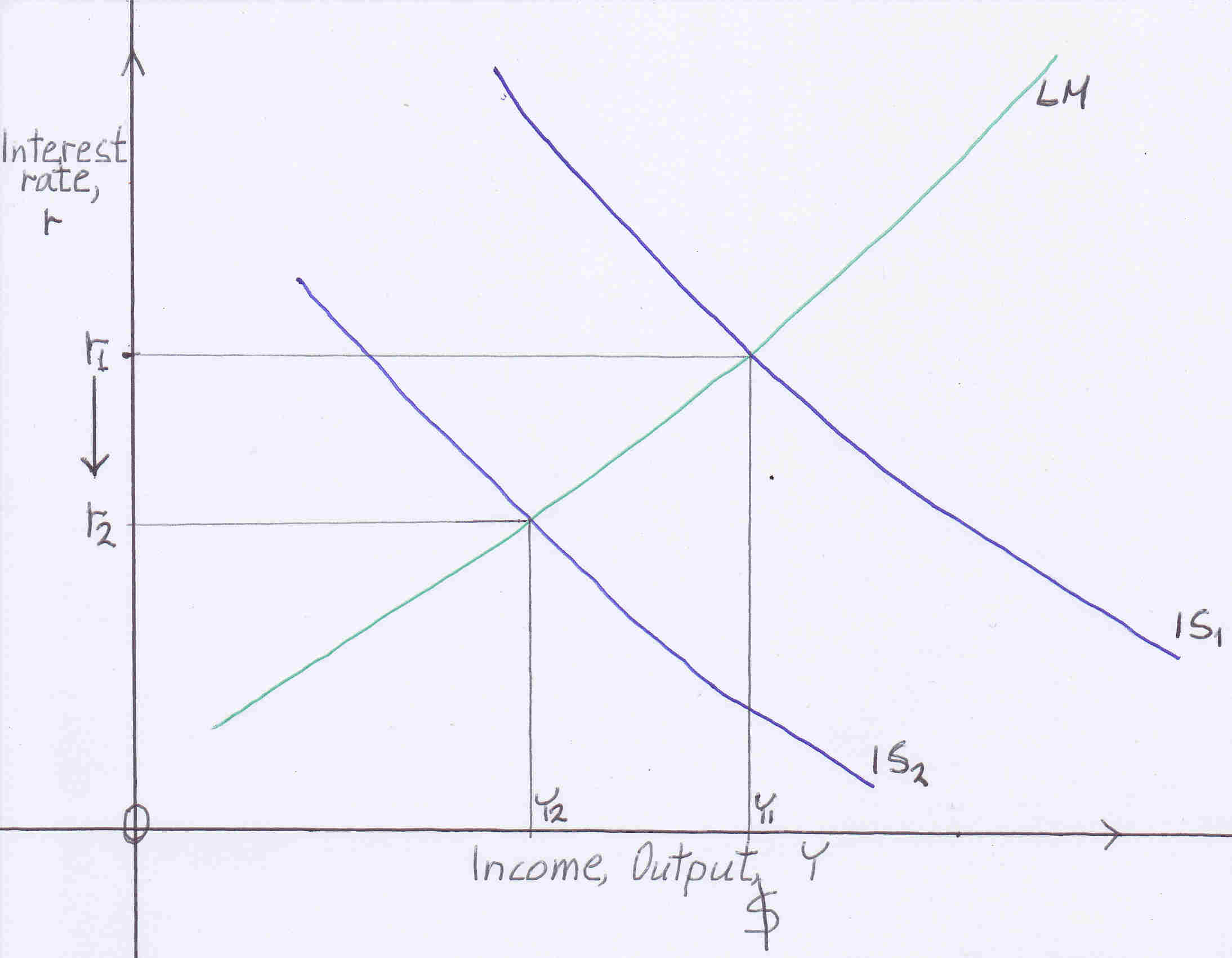 A tight fiscal policy shifts the IS curve down because National income Y is reduced. Government spending is one of the components of Y.
Figure 20
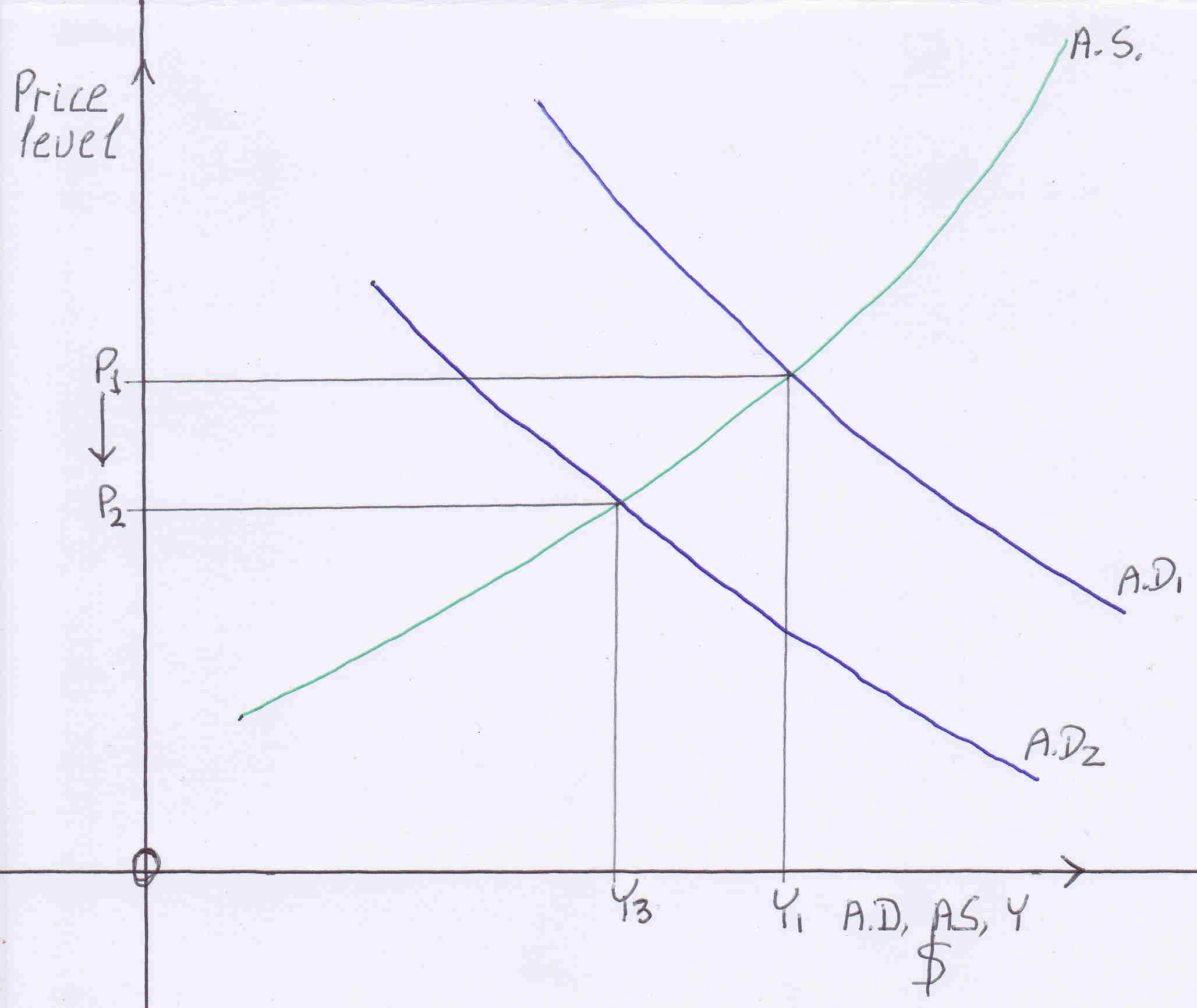 Government spending is reduced consequently aggregate demand is reduced, shifts down reducing Y to Y3.
In the above two graphs interest rate is reduced from r1 to r2 and price level is reduced from P1 to P2
Combat inflation
Figure 21
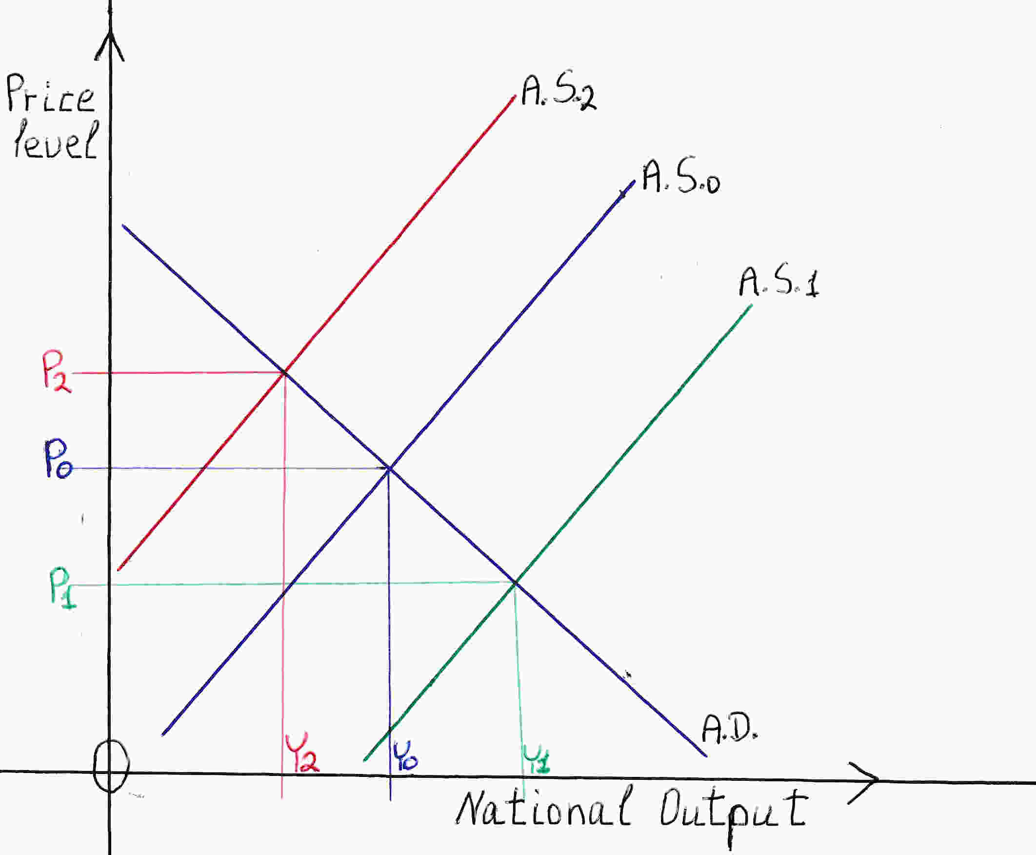
- If we find the causes of inflation we will find the solutions. The primary cause of inflation is the high price of oil (figure above AS0 shifts to AS2 Price increases from Po to P2, N.Y. falls from Yo to Y2). This is cost-push inflation. USA increase greatly the output of oil. Do not worry about tomorrow. Do not keep oil reserves in earth. Alternative sources of energy are advancing. You will end up having the oil in earth and not be able to get it out. Also you can agree with OPEC+ to reduce the price of oil. Low price of oil leads to reduced inflation and high economic growth (figure above AS0 shifts to AS1 Price decreases from Po to P1, N.Y. rises from Yo to Y1). A second cause of inflation is when aggregate demand exceeds aggregate supply. This is demand-pull inflation when unemployment is low.
- The pensioners can work earning simultaneously their pension and the salary of their work.
- All employers should be allowed to deduct from their taxable income the salaries of their teenagers employees under 18 years old. That is a second time: 2 times. The first is in the salaries of all employees the second as described above that is open an account with a debit entry for example tax deductions teenagers account. The corresponding credit entry of the second should be carried forward together with the retained profit. Encouraging employers to employ teenagers under 18 years old.
- All employers when they buy a computer for a teenager will record 2 double entries. The first credit Cash or Creditor (Seller of the computer) and debit Computers (asset). The second: credit tax gift computers for teenagers which will be carried forward with the retained profit and debit tax deductions computers for teenagers account which will be deducted from the taxable income. After 2 months of employment of the teenager a third double entry should take place: credit Computers (asset) account and debit the Computers giveaway to teenagers account which is an expense account. That is in 2 months the ownership of the computer passes from the employer to the teenager.
- Foreigners can work from their foreign countries using their computer to work for USA.
- Robot incentives: Abolish all taxes and duties on purchases of robots.
When a firm buys robots it can record a credit entry to an account : tax gift robots. This amount will be carried forward together with the retained profit account. The debit entry being tax deductions robots account will be deducted from the taxable income in one year or more.
In addition depreciation of robots will take place every year until the book value of this asset is zero or it is sold. - All the unemployed should declare at least one job that they are willing to work. Alternatively they should attend classes for acquiring skills, schools organized by the government. Those who declare a job should go and assist an employer of that job. The unemployed person should receive the unemployment benefit from that job. Those who are trained in a school will receive the unemployment benefit at the school. If there are unemployed who conform to neither of the above they should go to offices assigned by the government which act as an agent for finding work. There should be announcements of vacant jobs in that office where the unemployed should consider. Employers who seek unemployed for work should conduct that office and post invitations for work. The unemployed person after reading the invitations he has to sign a declaration that he read the invitations and receive the unemployment benefit from that office. This will be done weekly. If the unemployed do not turn up to receive it within 3 days he loses it. Unemployment benefit checks should not be sent to the home of the unemployed nor to their bank accounts. This measure reduces the black economy (figure above AS0 shifts to AS1).
- The government should not tax overtime (figure above AS0 shifts to AS1).
- All employees should be allowed to work more than one job if they want to. The job with the highest salary will only be taxed.
If the salaries of all the jobs of an employee when added, only then exceed the tax allowance then the sum of all his salaries is taxed. - Reduce the duration of the unemployment benefit from 6 to 3 months.
- Reduce the amount of the unemployment benefit.
- Import electricity via cables from other countries such as Canada reducing the price of electricity.
- Reduce transportation costs. The government should reduce the price of subway, buses and other transportation tickets as long as there is the thread of inflation.
- An exam and an essay including a cash flow should be required from those who want to start a business to those who pass the above a sum of $200.000- should be given by the government to start their own business. For example, the government gives 10 million to a university and asks to be distributed, all of it, to 50 graduates who want to start their own businesses (figure above AS0 shifts to AS1).
- Industries that are monopolies and there is room for competition the government should tax the monopolistic firm with higher taxes than the new comer firms (figure above AS0 shifts to AS1).
- The government should sell some of the land it owns, now that it is pricey, driving the price of immovable property down.
- As long as there is the thread of inflation the sales tax (or the V.A.T. in Europe on certain goods, food) should be abolished.
- The value of dollar should be raised let the dollar appreciate due to the interest rate hikes. Thus, all imports will be cheaper including oil all exports will be dearer forcing the US manufacturers to lower their prices and focus in the US market where there will be abundant low priced goods. The appreciation of the dollar should be done in steps over a period of time until inflation is controlled. The appreciation is a good measure it certainly lowers inflation but it has a temporary effect it does not fight inflation. What fights inflation is the rise of interest rates and a tight fiscal policy as explained previously.
- Abolish all import duties at least as long as inflation is high. This will drive inflation down. If all duties are abolished the trade will flourish. Import duties do not reduce imports the trade balance does not improve because import duties cause the dollar to appreciate causing the net exports (NX) to remain the same. Other ways for appreciating the currency should be adopted.
National Income = GDP = C+T+S = C+I+G+NX
(S+T-G) - I = NX
S + T -G = Total Savings
ST - I = NX
Net Exports equal Savings - Investment
For example if G (government spending) increases, Savings (S) decrease, net exports (NX )decrease. When G increases a part of this increase is allocated to spending on imports. Thus, NX decrease.
When the US dollar depreciates NX increase because imports become dearer exports become cheaper. As exports and domestic production increases GDP increases Savings increase (Savings=GDP-C-G).
As mentioned above S and NX are interrelated: S affect NX and vice versa. - The government should rent land it owns to individuals for farming and agriculture.
- Abolish quotas and restrictions on food imports, as long as the inflation is high, for the price of food to go down.
- Banks charge higher interest on people who borrow for consumption, cars, furniture, household equipment and so on.
Charge the lowest possible interest on investment. - Increase the number of green cards the USA issues, for example, to Ukrainians.
- Mexicans may be given non immigrant visas lasting 2 years.
- Now that there is shortage of wheat, sunflower seeds can be used for producing bread instead of oil. More olive oil can be produced instead of eating the olives.
- The government should demand from its civil servants to increase their productivity promising to reduce the working hours. When the working hours are reduced to 38 per week the government will say well done productivity has increased the hours will be reduced to 35 per week. I think Mr. Berluskoni has done it in Italy with great success. One day people will work 35 hours or less per week. Besides when you work you do not consume.
- The government should demand all employers of 8 or more employees to announce a most productive employee of the month and give her/him a prize of at least half of the average monthly salary of all employees. The employer should announce the prize beforehand.
- Employers who employ more than 30 employees should provide their employees a canteen with good food, fruits and pleasant music.
- All employers should demand their employees to pray the Lord's prayer: Our Father and then pray: "Lord Jesus Christ thank you for the job you have given us make us happy and productive." Just before starting work in the morning.
- Big firms must have a trainer, dietitian, Christian therapist, physician for all their employees a small proportional sum be deducted from the salary of every employee to reward the above.
- Employers should take out all their employees for dinner, socializing, dancing once a month.
- If the commissions and charges on exchange of currencies on trade, visible and invisible, are abolished all imports and all exports will become cheaper. This will have a negative effect on inflation. It will also encourage trade. I am not talking about money transfers or any other exchange of currency other than all trade. The banks are the backbone of the economy. Governments should negotiate with the banks to increase the net interest rate spread (difference between lending and borrowing rate) or compensate the banks for all the commissions and charges foregone.
Do not be overwhelmed these are just some ideas to reduce inflation. What matters is what God and most people want.
Deficit financing
We all want lower taxes and a generous government. How can we achieve this without causing inflation to rise?
As Professor William H. Branson says in his book Macroeconomic Theory and Policy there are 5 ways for a government to finance its deficit:
1. The US government can sell bonds to the nonbank public. It is rather inflationary.
2. The US government can sell bonds to the commercial banks. Thus, the banks pay the US government and reduce lending to the private sector. It is rather inflationary.
3. The US government reduces its demand deposits(money it has in the commercial banks) at the commercial banks. It is inflationary.
4. The US government issues and sell bonds to the Federal Reserve System which Fed prints money, buys the bonds giving the money to the US government. It is highly inflationary.
5. The US government takes money from the Fed. It is highly inflationary.
A.D. > Aggregate Supply
Lower taxes and a generous government without causing inflation to rise is accomplished by a tight monetary policy: The Fed sells bonds increasing the interest rates.
Inflation takes place when A.D. exceeds Aggregate Supply (A.S.). Therefore to control inflation either A.D. should be decreased (tight monetary and fiscal policies) please see Figure 20, for only tight fiscal policy, National Income decreases from Y1 to Y3 thus in this case the economy enters recession or A.S. should be increased please see Figure 21 National Income increases from Y0 to Y1. In this case the economy is booming while Prices fall.
In this essay supply-side economics are studied emphasizing predominantly how A.S. is increased see passages Long run aggregate supply curve shifts, Combat inflation (increase of the four factors of production: labor, land, capital, entrepreneur).
Governments, the Fed, policy makers are right because the economy is dynamic: A.D., A.S. are ever-changing. When A.D. is fast-paced tight monetary and fiscal policies should be adopted together with measures to increase A.S. as mentioned above. If this A.D. is not controlled at some point the economy will reach its full capacity and then inflation will soar.
Please, bear in mind that the real interest rate(r, see graphs) is now negative.
I mentioned many measures to combat US inflation the most important is please pray that inflation is reduced without hurting you or the economy and you may prosper. Pray that the world economy has a soft landing and there will be no third world war.
Christmas is a time when kids tell Santa what they want and adults pay for it. Deficits are when adults tell the government what they want and their kids pay for it.
Richard Lamm
Bibliography
Macroeconomics, N. Gregory Mankiw
Macroeconomics, Rudiger Dornbusch, Stanley Fischer, Richard Startz
Macroeconomic Theory and Policy, William H. Branson
Macroeconomics, Paul A. Samuelson, William D. Nordhaus
Macroeconomics, Dernburg, McDougall
Principles of Economics, N. Gregory Mankiw
An introduction to Positive Economics, Richard G. Lipsey
Economics, David Begg, Stanley Fischer, Rudiger Dornbusch
Economics, Paul A. Samuelson, William D. Nordhaus
Fundamental Methods of Mathematical Economics, Alpha C. Chiang
Microeconomic Theory A Mathematical Approach, James M. Henderson, Richard E. Quandt
Price theory and applications, Jack Hirshleifer
The author is an economist, a graduate from City, University of London
Fast and accurate way to calculate the monthly payment of a loan
Enter the amount of the loanEnter the annual interest rate of the loan, for example if it is 4% enter 4
Enter the number of years to repay the loan
Lord our God, our all-powerful Father, You who gave birth to wisdom let all the words in this essay be Yours and not mine. In Jesus' name. Amen.
Go to the Home page.
Go to the Early Jewish Writings.


