Individual income can grow as fast as productivity rises.
Alex Berenson
Jesus Christ is Lord of money:
Matthew 17:24-27: "After Jesus and his disciples arrived in Capernaum, the collectors of the two-drachma temple tax came to Peter and asked, “Doesn’t your teacher pay the temple tax?”
“Yes, he does,” he replied.
When Peter came into the house, Jesus was the first to speak. “What do you think, Simon?” he asked. “From whom do the kings of the earth collect duty and taxes—from their own children or from others?”
“From others,” Peter answered.
“Then the children are exempt,” Jesus said to him. “But so that we may not cause offense, go to the lake and throw out your line. Take the first fish you catch; open its mouth and you will find a four-drachma coin. Take it and give it to them for my tax and yours.”"
Jesus Christ is the richest Man -GodMan- in the universe. He owns everything. A proof, He is the reigning King coming to earth the second time as in the scriptures, Holy Bible:
Matthew 25:31-34:
""When the Son of Man comes in His glory, and all the holy angels with Him, then He will sit on the
throne of His glory. All the
nations will be gathered before Him, and He will separate them one from another,
as a shepherd divides his
sheep from the goats. And He will set the sheep on His right hand, but the goats
on the left. Then the
King will say to those on His right hand, "Come, you blessed of My Father,
inherit the kingdom prepared for
you from the foundation of the world."""
Jesus Christ created everything there is nothing that Jesus Christ did not create. He created everything out of Himself. Before the beginning of the universe Jesus Christ was with His Father. There was no space, no matter, no time, just love. Jesus Christ created even satan. Therefore He owns everything He is the only creator. He is God.
Economics is the study of how consumers maximize utility, how producers maximize profit, how governments maximize welfare of their citizens and how investors maximize return. The law of diminishing returns gives us that for every unit of additional output produced, the addition to total cost increases more rapidly. Therefore, in perfect competition the supply curve, in units of output, is a positively sloped curve that as output increases becomes steeper. When we ask the firms how much they are willing and able to produce at different prices we derive the supply curve done in an empirical fashion. In this essay the output in units of a good or service is multiplied by its corresponding price to derive output in value, money, number of dollars. Perfect competition, monopoly, monopolistic competition, oligopoly comprise the economy and are all added up to define the short run aggregate supply curve (srasc). It is explained why and when srasc shifts and has that slope.
Marginal cost
Profit maximization
Perfect competition
Monopoly
Technical information
Monopolistic competition
Oligopoly
Adding up all markets
An example with figures
Shifts and slope of srasc
Conclusion
Marginal cost
Marginal cost(M.C.) is the cost incurred in producing one additional unit of output. It is the addition to Total cost(T.C.) for producing 1 additional unit of output. The law of diminishing returns gives us that the marginal cost increases at a faster pace. Why?
When we add input to produce more goods, for example, when we add workers (labor) there comes a time that the output does not increase by the same proportion of the additional labor employed. Too many workers collide, their relative space decreases they are more disorganized. The output they produce is not proportional to the input of labor. For example, a factory building with the machines has a capacity of 100 workers if the workers are increased to 200 the output will not double. Workers are not the only variable cost. If the firms' demand for raw materials increases the price of raw materials will increase thus marginal cost progresses. Therefore, to produce one additional unit the cost (wages) is increasing at a faster pace. As output increases the cost is rising at a steeper rate: diseconomies of scale. The following diagram illustrates it:
Figure 1
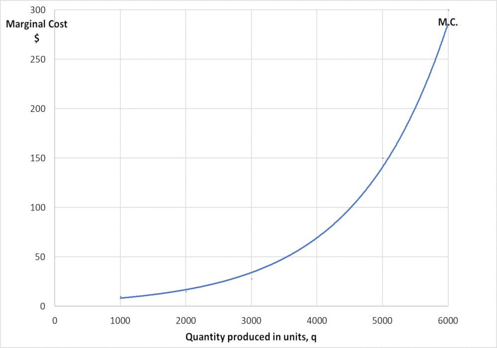 As quantity produced increases the M.C. is steeper.
Profit maximization
From the graph below we conclude the M.C. curve is the supply curve in the short run in perfect competition we explain below. Please note that the average revenue(A.R.) curve (A.R. is the revenue that is earned by the producer on selling each unit of output. It is the total revenue divided by the total output. It is the price of the product.) and the marginal revenue(M.R.) curve (M.R. is the change in total revenue by selling one additional unit of output) are the same, parallel to the x-axis only in perfect competition(pc). The graph below is for all markets.
Figure 2
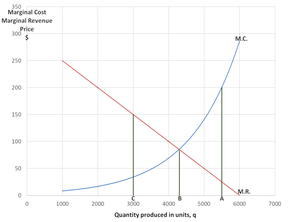 From figure 2 at output A, M.C. is more than the marginal revenue(M.R.) which in perfect competition(M.R.=A.R=price) is the price. M.C. is greater than the price. The firm loses money so it will produce less. At output C, M.R. is greater than M.C. the price of one unit of output is $150- the M.C.=$33-. The firm gains profit and it will produce more to gain more profit until M.C.=M.R. at B (see figure 2). If it produces more than B M.C.>M.R. the firm loses money. The firm will produce at B where Price=M.C. The firm produces where the price of the product=M.C. it produces that output. Therefore, the M.C. curve is the supply curve in perfect competition(pc). At a given price how much it will produce: supply curve.
In markets except pc: as output increases M.C. increases due to diminishing returns. At higher M.C. there is a higher M.R. curve to intersect it which leads to a higher A.R. curve(M.R. and A.R. are interrelated) which A.R. is the demand curve the price: Higher output higher price: figure 8
In economic theory price is always determined by M.C. curve, M.R. curve and A.R. curve which is the demand curve.
Perfect competition
An equation with actual figures of the Price (P) and quantity in units (q) of the supply curve of perfect competition is:P= q280-1.7q + 62
The graph of P= q280-1.7q + 62
is as follows:
Figure 3
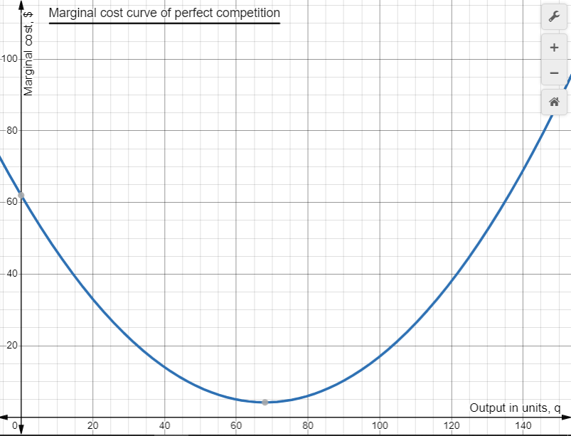
Now, the correct supply curve is to relate Price and output in money, dollars, because you can not add the output when it is in units of a good or service. Can you add apples and televisions? Also, the National Income or National Output or GDP is expressed in money, dollars.
To find the supply curve of the above equation we multiply q (quantity in units) by P (price). Output in dollars= Pxq => q= OutputP = yP substituting in the equation (Price - quantity):
P= q280-1.7q + 62 where q= yP:
We have:
P3 - 62 P2- y280+ 1.7py = 0 , equation of supply curve, Price, Output in value, dollars.
Graph of perfect competition supply curve in dollars: curve to the right.
Figure 4
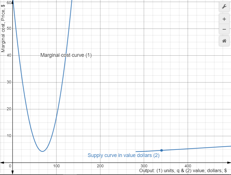
The equation of the supply curve in value: P3 - 62 P2- y280+ 1.7py = 0 consists of other curves in addition to the curve above which are eliminated because the marginal cost curve, in units, is the supply curve for only its positive slope the right part which corresponds to the supply curve in value output $ shown. (The marginal cost curve is the supply curve for values greater than the intersection between the marginal cost curve and the average variable cost curve(at its minimum)).
The supply curve in dollars is almost horizontal its slope is small. At first side we conclude that price is sticky in the short run. However, look at the marginal cost (left) - supply curve of pc in units: It is steep (the calibration of the x and y axis is different from figure 3 to be able to compare the graphs of supply in units with supply in output, dollars).The supply curve in dollars is shallow because each output in units is multiplied by its corresponding price. A breakthrough in macroeconomics.
Now we derive the supply curve in dollars for perfect competition:
P = apcq + bpc , q: quantity in units, P: Price, apc and bpc: parameters - equation of marginal cost curve simplified for perfect competition
y = Pq => q = yp , y output in value, dollars
∴ P = apc yp+ bpc
P2 = apcy + bpcP
∴ y = P2apc1- bpc1apc1P , firm 1 - add all firms' curves
y = P2apc2- bpc2apc2P , firm 2
where 1 apc= 1 apc1+ 1 apc2+ . . .
bpc apc= bpc1apc1+ bpc2 apc2+ . . .
We solve for P:
Monopoly
In monopoly, there is no unique relation between market price and quantity supplied. There is no distinct supply curve under monopoly. Yet when the demand curve shifts to the right (increases) there is a relation between increase in prices and increase in quantity supplied as the following graph shows under the assumption that the demand curve shifts parallel:
Figure 5
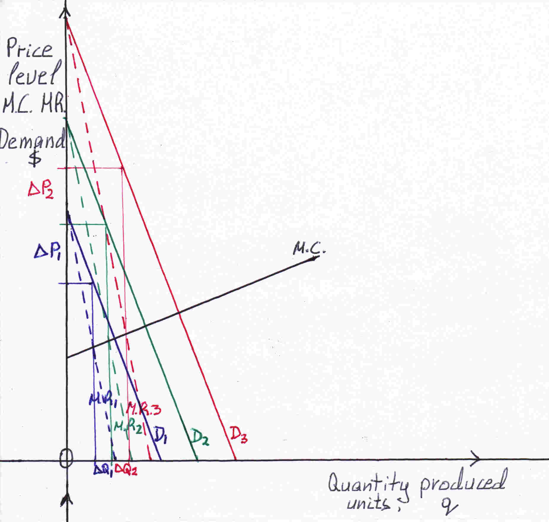 The monopolist produces that output where M.C.=M.R. to maximize profit as it was explained. From the graph above you can see the output determined is at the intersection of the M.C. curve (black line) and the M.R.1, M.R.2, M.R.3 curves (dotted lines). The monopolist sets the price at which consumers are willing to pay at the determined output the demand curves D1, D2, D3. Where the output meets the demand curve we get the price. From the above graph you can see that the change in quantity ΔQ increase is less than the change in price ΔP (increase). The price compared to quantity increases at a larger rate.
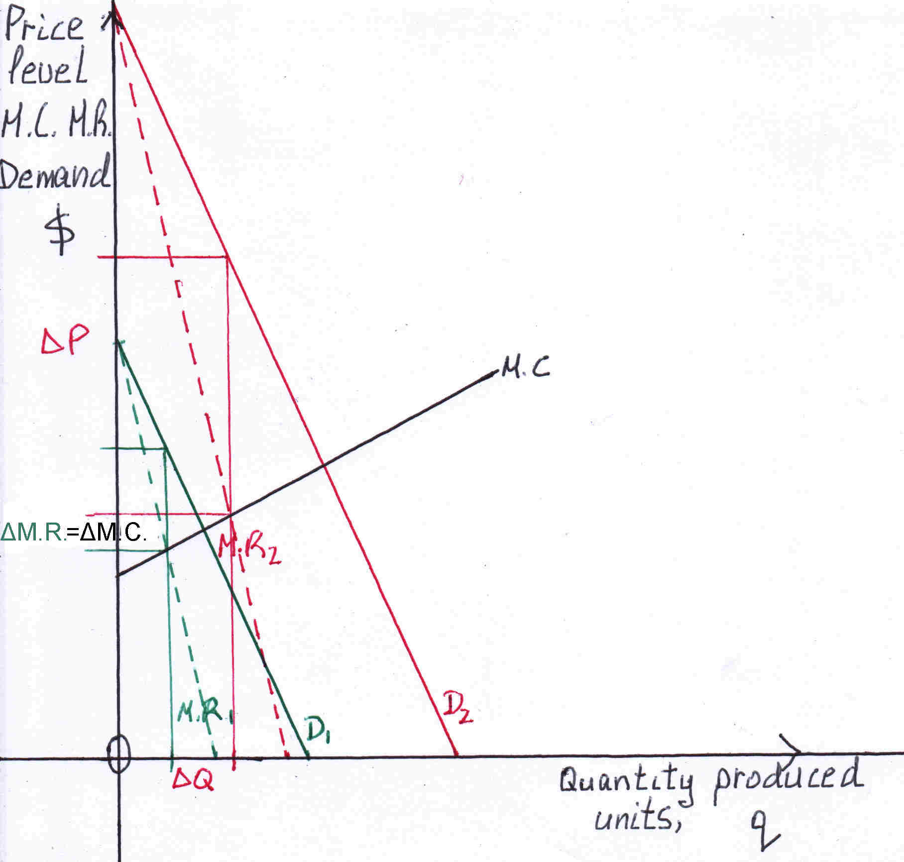
Please see figure 6, below.
The demand curve is the average revenue(A.R.) curve:
A.R.=Total revenue/quantity = price✕quantity/quantity = Pq/q = P
Let the equation of the demand curve be PD=mq+c where m: slope, c: intersection to the y-axis or Price-axis
Marginal Revenue= d(T.R.)/dq = d(PDq)/dq = d(mq2 + cq)/dq = 2mq+c
The slope of the demand curve is m and is negative. As proved the slope of the M.R. curve is 2m it is twice as steep.
The A.R. curve meets the q axis:
0=mq+c
mq=-c =>q=-c/m
The M.R. curve meets the q-axis:
0=2mq+c =>q=-c/2m
The horizontal distance from(0,0) is half for the marginal curve. When M.R. is zero it intersects the q-axis at q=-c/2m at that q the A.R.= mq+c= m(-c/2m) + c= c/2
When M.R.=0 A.R.= c/2
A.R.=y
M.R.=x
M.C.=z
mc: slope of the M.C. curve
cc: intersection of the M.C. curve to the y-axis or Price-axis
x1=2mq1+c1
x2=2mq2+c2 => Δx= 2mΔq+ Δc
At the two points of intersection between M.R.s and M.C. we have:
z1=mcq1+cc
z2=mcq2+cc => Δz= mcΔq
∴Δz= Δx
∴mcΔq= 2mΔq+ Δc
∴Δc= mcΔq- 2mΔq —✱
y2= mq2+ c2
∴Δy= mΔq+ Δc
From just the above equation and from ✱: Δy= mΔq+ mcΔq- 2mΔq
∴Δy=mcΔq- mΔq
∴Δy= (mc -m)Δq
∴ΔP= (mc -m)Δq
∴ΔP/Δq= mc -m
∴P= (mc -m)q+ bm
∴P= amq+ bm
am= mc- m, mc>0 the slope of the marginal cost curve, m<0 the slope of the demand curve which is negative so -m is positive therefore am>0, bm is a number
Figure 6
 Why is the demand of a monopolist steep, |m| is high?
Because consumers cannot switch to another brand it is monopoly. A change in price brings a small change in quantity sold and thus produced. Therefore we assume that the demand curve shifts and not pivots(elasticity of demand changes dramatically) and also the M.C. is a straight line that does not shift (please see figure 5).
Figure 7
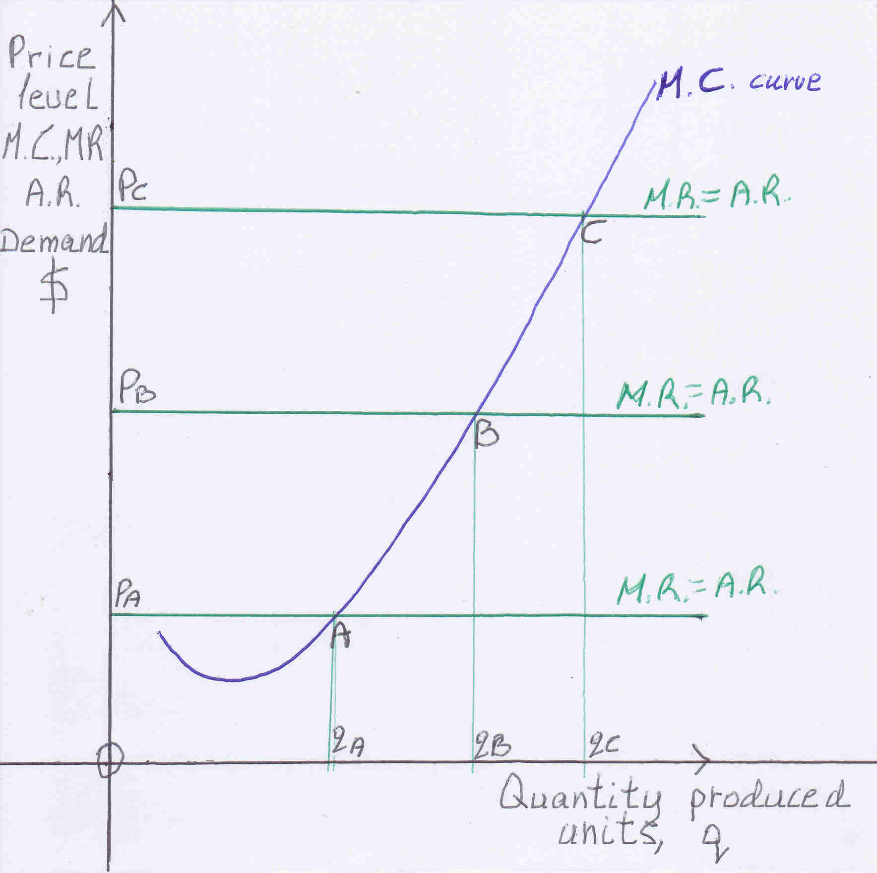 As explained previously the perfect competitive firm will produce that output where M.R.=M.C. to maximize profits. The M.R. curve is the same as the A.R. curve which is the demand curve and it is parallel to the x-axis and to the other demand curves. The points of intersection between M.R. curves and the M.C. curve describe the supply curve for example at output qA the price is PA at output qB the price is PB and at output qC the price is PC but these points as it is illustrated is the M.C. curve: points A, B, C.
Figure 8
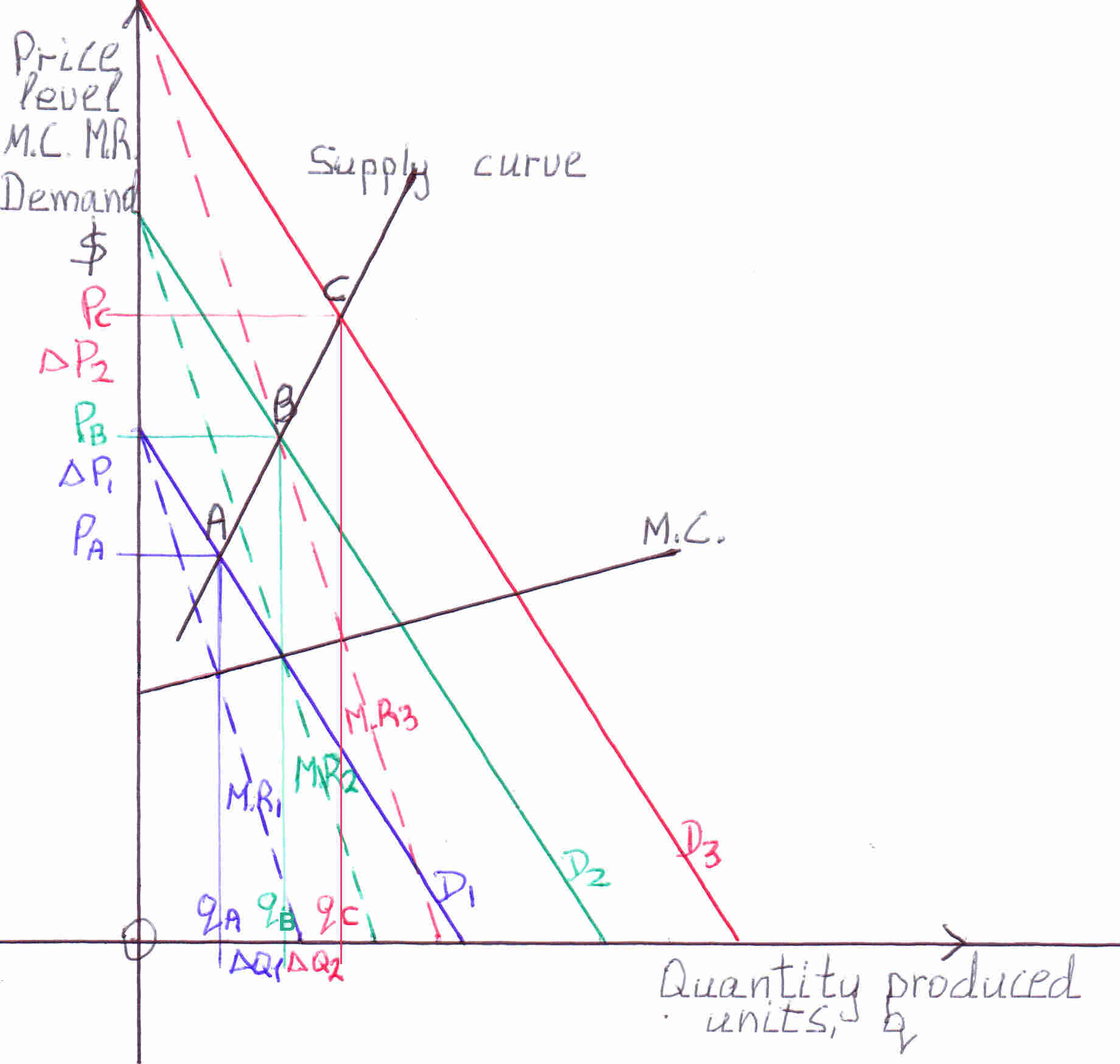 In monopoly the monopolistic firm will produce the output where M.R.=M.C. to maximize profits where M.C. curve intersects the M.R. curve (dotted line). At that output we find the price we move upwards vertically until we meet the demand curve, D, of the monopolistic firm. There, is the price of the product. Therefore, at output qA the price is PA. At output qB the price is PB and at output qC the price is PC. The line which connects these points A, B, C,: (qA, PA) (qB, PB) (qC, PC), see the graph above figure 8, is the supply curve of the monopoly the philosophy is the same as in perfect competition. Of course, we assume that the demand curve shifts parallel to the previous demand curve. If it pivots we connect the points as done above and we will find the supply curve.
From the above calculations we have P= amq + bm equation of supply curve in monopoly of Price, output q in units.
The principle is the same as in perfect competition:
Monopolistic competition
In monopolistic competition there are many firms with freedom of entry and exit (competition). Yet each firm has some power over price because each sells a product that is somehow different from the firm's competitors (monopoly). The demand curve is rather elastic because there are substitute products from other firm competitors: As it was mentioned in monopoly the demand curve does not pivot because the elasticity of demand normally does not change it is a monopoly, consumers cannot switch to other goods. In monopolistic competition, however, the demand curve of a firm pivots because consumers can consume other similar products as the graph below demonstrates.
Figure 9
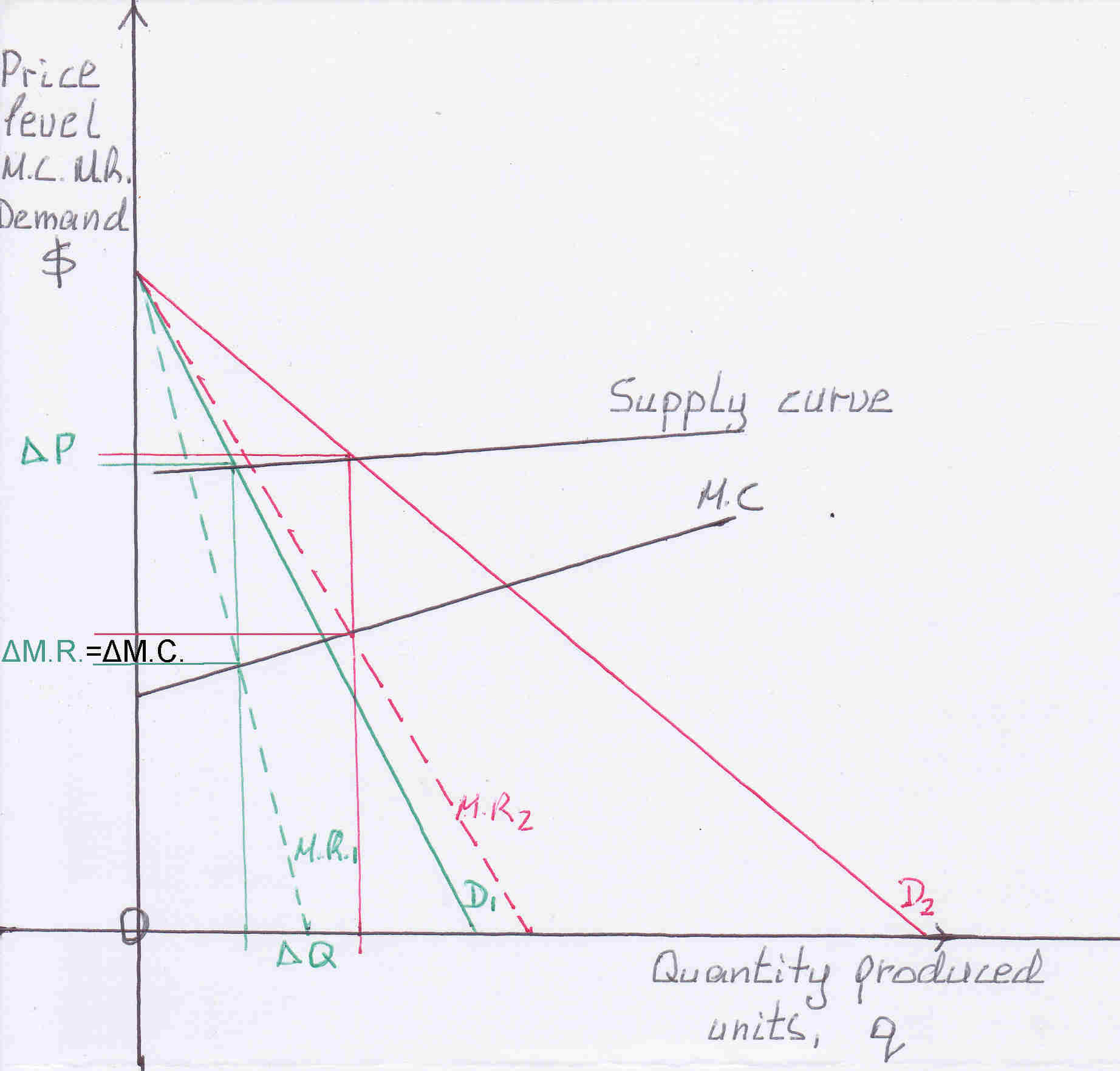 When the demand curve pivots from D1 to D2 there is a small change in price ΔP.
We showed in monopolistic competition(mc) that variation in quantity changes the price.
Now let:
A.R.=y
M.R.=x
M.C.=z
m1: slope of demand curve 1, D1
m2: slope of demand curve 2, D2
mc: slope of the M.C. curve
c: intersection of the A.R. & M.R. curves or y & x curves to the y-axis or Price-axis
cc: intersection of the M.C. curve or z curve to the y-axis or Price-axis
y1= m1q1 + c
y2= m2q2 + c
∴Δy= m1q1 - m2q2
x1=2m1q1+c
x2=2m2q2+c
∴Δx=2m1q1-2m2q2
z1=mcq1 + cc
z2=mcq2 + cc
∴Δz=mcΔq
But Δz=Δx see figure above
∴ mcΔq = 2m1q1 - 2m2q2 —✱
But Δy= m1q1 - m2q2
From just the above equation and from ✱: Δy = 1 2mcΔq
∴y = 1 2mcq + bmc
P = 1 2mcq + bmc
P = amcq + bmc
∴amc = 1 2mc, mc: slope of the Marginal Cost curve, bmc is a number
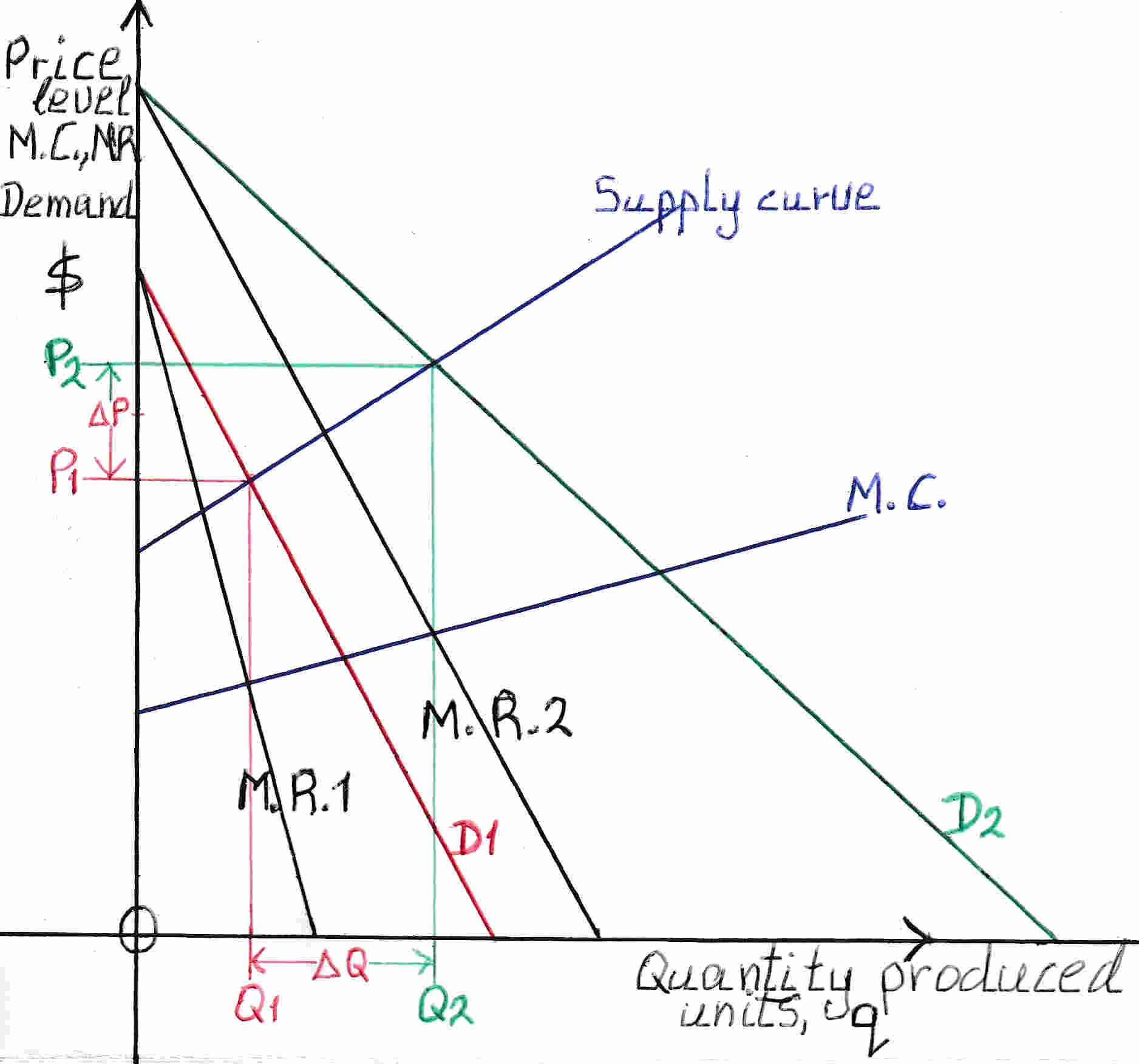 What if the demand curve moves randomly like in the graph above from D1 to D2:
Profit maximization is when M.R.=M.C.
Now let
Cc: intersection of the marginal cost curve to the y-axis.
C1: intersection of the initial demand curve D1 or A.R.1 curve and M.R.1 curve to the y-axis.
C2 intersection of the subsequent demand curve D2 or A.R.2 curve and M.R.2 curve to the y-axis.
mc: slope of the marginal cost curve.
m1: slope of the initial demand curve D1 or A.R.1 curve.
m2: slope of the subsequent demand curve D2 or A.R.2 curve.
Q1, P1: Point 1
Q2, P2: Point 2
We find Point 1
M.R.= M.C.
2m1q1 + C1 = mcq1 + Cc
2m1q1 - mcq1 = Cc - C1
Similarly we find Point 2
P= amcq + bmc - equation of monopolistic competition supply curve of Price, output q in units.
What if the demand curve moves randomly again? We find Point 3 by equating M.R.=M.C. as done above. We, then, do either regression analysis (best line through the points) or interpolation (best equation that describes the points) and we find the best possible equation of Price and quantity. We can take real, actual monopolies, all firms in monopolistic competition of a particular product and collusive oligopolies and observe the relationship between Price and quantity produced.
Oligopoly
In oligopoly few firms compete with each other. Each firm has enough power so that it cannot be a price taker(take price as given), but it is subject to enough inter-firm rivalry that it cannot consider the market demand curve as its own. This is probably the dominant market structure outside agriculture and basic industrial materials. In non-collusive oligopoly the price is sticky:
Figure 11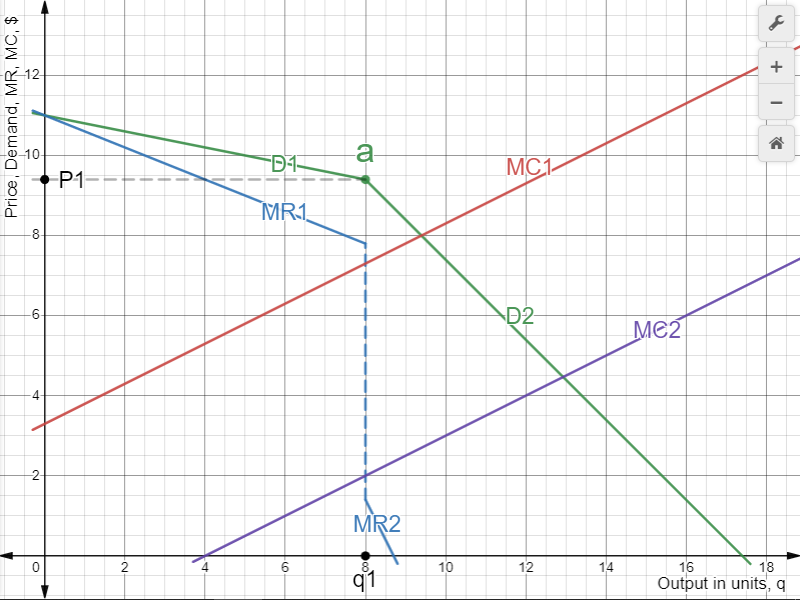
In the figure above the oligopolistic firm is assumed to be selling q1 units at a price of p1. It then considers altering its price and it makes two key assumptions. First, it assumes that if it cuts its price, all of its competitors will match its price cut. Its demand will then expand along the relatively steep curve below a, which indicates the effect of the firm's price cut when its share of the market is unchanged. Second, it assumes that if it raises its price, above p1, none of its competitors will raise theirs. Its demand for prices above p1 thus contracts along the relatively flat curve indicating the effects of raising prices with a declining market share. To summarize, above price p1 the competitors will not increase the price thus the firm loses a lot of demand: a small increase in price leads to a large decrease in demand the demand curve is flatter. At price below p1 the competitors will also reduce the price there will be no change in the firm's demand, competitors follow suit therefore the demand curve is steep a change in price brings a small change in output. Therefore, in the above figure 11 in non-collusive oligopoly M.C. changes(shifts) the price remains the same.
Figure 12
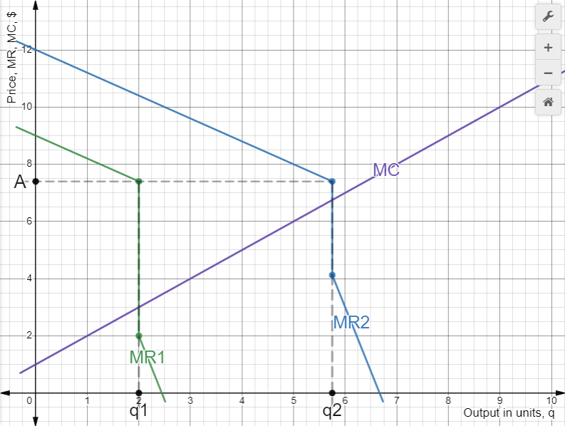 See the figure above: as demand increases the demand curve and thus the marginal revenue(MR) curve shifts from MR1 to MR2 the quantity changes from q1 to q2 but MR(point A) remains the same because price remains the same.
From the above figure 12 in non-collusive oligopoly as quantity changes price is constant.
In order to find the overall supply curve of oligopoly we use the weighted average method because it is the best under the circumstances. The classic solution is to solve for q, output, and then add them up. Now, because non-collusive oligopoly has a fixed price the outcome will be P= fixed price of non-collusive oligopoly which is wrong because the output of non-collusive oligopoly is not infinite. Suppose all the output of non-collusive is $5,000,000= the parallel line to the x-axis at price Pnon-collusive oligopoly stops at $5,000,000=. I thought of using ranges for example 0<= non-collusive curve <= 5,000,000= and then the curves of the other firms. Is non-collusive at the beginning, middle or end? In reality goods of non-collusive are supplied randomly with the goods of other firms.
Examples of collusive oligopolies
OPEC+ oil industry
De Beers diamond industry
Airline industry
Pharmaceutical industry
Cement industry
Therefore, the overall supply curve of the oligopoly market Price, output in units q is:
P= aoq + bo
Adding up all markets
y = P2a- baP short run aggregate supply curve (srasc)where 1 a= 1 apc+ 1 am+ 1 amc + 1 ao
ba= bpcapc+ bm am+ bmc amc+ bo ao
Y is the potential output of the economy. When Y potential output or natural level of output increases Y increases by the same amount. Incorporating Y natural level of output in our model Yt1 = Y at time t1 at the beginning when the calculation of the parameters a and b are made:
Yt1 = f(P) = f2(P) + Yt1
Y = f(P) = f2(P) + Y
f2(P) = Yt1 - Yt1
f2(P) = Y - Y
Yt1 - Yt1 = Y - Y
Y = Yt1 + Y - Yt1
Y = f(P) + Y - Yt1
Price that is not at time t1 is deflated (divided by the GDP deflator) to time t1. Also, Y natural level of output and Y national output are deflated to time t1.
An example with figures
P = 1.5q + 74.5 - equation of marginal cost curve, supply curve, simplified using regression analysis of perfect competition, output in units (number of goods produced)
P = 2.1q + 64.3 - supply curve of monopoly
P = 1.1q + 43.9 - supply curve of monopolistic competition
P = 1.5q - 27.5 - supply curve of Oligopoly
Y = P2a- baP + Y - Yt1
where 1 a= 1 1.5+ 1 2.1 + 1 1.1 + 1 1.5 = 2.7186
b a= 74.51.5+ 64.3 2.1 + 43.91.1 - 27.51.5 = 101.8615
Y = Yt1 = 10,000.00
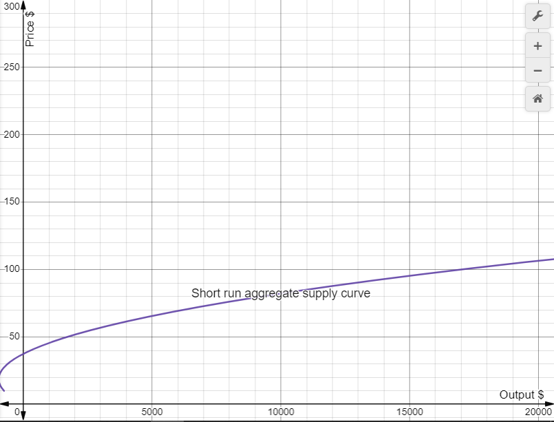
Y = 2.7186P2 - 101.8615P + 10,000.00 - 10,000.00
Y = 2.7186P2 - 101.8615P , its graph is as below
Figure 13
Shifts and slope of srasc
Figure 14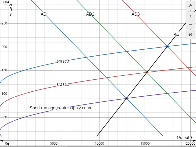
The long run is many short runs added together. For the long run supply curve to be vertical it means that at a certain short run the short run aggregate supply curve shifts upwards. The marginal cost curve describes how the marginal cost changes as units of output produced increase. The more units of output produced the more labor is employed (which increases more rapidly than the output produced (law of diminishing returns)) the more wages expenses rise (wage per hour remains the same): movement along the Marginal Cost(MC) curve. If wage per hour increases it means with the same labor and thus the same units of output the marginal cost increases. This a shift of the MC curve upwards. When the marginal cost curve shifts upwards the short run aggregate supply curve (srasc) shifts upwards see When marginal cost changes. When does the wage per hour increase (srasc shifts upwards)? When the National Output exceeds the natural level of output (full employment) because the labor becomes more scarce. At high levels of output when the AD curve shifts to the right, increases, the output increases demand for labor increases, labor is scarce, wage per hour increases srasc shifts upwards as in Figure 14. The supply curve is then the black line in Figure 14 that connects these points, AS that is why srasc turns upwards as it was explained continuously in deriving the srasc 1 (essay 1).
The actual srasc is like the Figures 13 & 14. Economists examining empirical evidence observe the srasc turns upwards. This is because the actual srasc (Figure 13) shifts upwards when AD curve shifts to the right and when the output exceeds the natural level of output Y. This actual srasc (Figure 13) takes place when wages remain the same. When wages rise marginal cost curve shifts upwards causing the srasc to shift upwards (Figure 14) because of: 1. see explanation above and 2. When marginal cost changes. The slope of srasc, as illustrated, is small not because the price is sticky but because every output is multiplied by its corresponding price to derive the srasc in value, money, dollars.1. A consumer maximizes utility (satisfaction)
2. A producer maximizes profit
If either of these two laws do not hold the whole economic theory collapses. Because Economics is based on laws, like Physics, Mathematics is an indispensable part of Economics. Young people if you want to be top Economists you have to be good in Mathematics if you are not do not pursue Economics.
Why am I writing all these words because the slope of the srasc depends on profit maximization: the output producers are willing and able to produce is where MR = MC therefore the slope of the srasc depends on the slope of the MR curve and MC curve (when the slopes of MC and MR change output supplied, price change). The MR curve has twice the slope of the demand curve which demand curve dictates the price. In perfect competition(pc) the supply curve is the MC curve and pc is taken into account in this model. The slope of the MC curve, (and supply curve in pc) depends on the level of wages. Higher level of wages make the MC curve steeper because to produce one additional unit in the short run labor is increased. The higher the level of wages the steeper (higher slope) the marginal cost is (wages are high but do not increase or decrease). Another factor is how labor intensive is the production. If production can increase without increasing labor it is zero labor intensive. Therefore, the slope of the MC curve (and supply curve in pc) depends on two factors level of wages and price of raw materials.
All the other monopoly, oligopoly, and monopolistic competition the output supply and the price depend on the MC curve and the demand curve of the products. Formulas have been developed in these essays of the supply curve which show that the slope of the MC curve and the slope of the demand curve determine the slope of the srasc in monopoly, monopolistic competition and oligopoly(same as monopoly). The higher the absolute slopes of the demand curve and MC curve the higher the slope of the srasc as illustrated. If the demand curve is elastic(low absolute slope) the srasc is elastic (low slope). To summarize the slope of the srasc depends on:
1. the elasticity of demand of the goods and services. If the demand curve is elastic the srasc becomes more elastic.
2. the slope of the MC curve (directly proportional to some extend). The slope of the MC curve depends on the level of wages and the price of raw materials.
3. the method srasc is derived: every quantity supplied is multiplied by its corresponding price. The higher the price the higher the value in dollars of the output (horizontal axis, it moves to the right) therefore the srasc becomes almost horizontal, flatter.
Equation of srasc:
P = 1 2(b + √ b2 + 4a(Y - Y + Yt1) )
The slope is inversely proportional to the square root of Y (National Output/Income). The higher the Y the smaller the slope, as Y goes to infinity the slope goes to zero. This contradicts the findings of essay 1 and empirical evidence which point out to a rising srasc.. The above slope is for one srasc while the above findings are for more than one srascs because at high outputs the srascs shift following the path of the black line AS as in figure 14 and as explained before. In the medium and long run the srasc shifts.
The srasc is derived microeconomically which is added up to reach the aggregate macroeconomically. While the AD curve is derived purely macroeconomically. Why couldn't we add the demand curves of products like we did in aggregate supply? Because of continuous shifts of the individual demand curves caused by macroeconomic factors. For example if the government prints and floods money in the economy AD is increased greatly.
AD = C + I + G + NX (macroeconomics).
Why srasc is derived microeconomically? Because aggregate supply depends on Capital K, Labor L, and technological progress A. In the short run Capital K, is fixed (K: buildings, machinery). Also, in the short run technological progress is fixed. Even if you start now you can not produce robots or AI programs in 3 - 4 months to increase aggregate supply (AS).
Y = AF(K, L) - (Y = AS, A = technological progress fixed, K = Capital fixed, L = labor). Labor employed can vary in the short run and this model takes labor as variable.
Conclusion
In conclusion, it is sad that Economics is one of the least developed sciences for the last 87 years unlike Physics, Astronomy, Medicine and others. In the 1930's there were readily available goods the shelves were full and overflowing and people were not able to buy them, the demand was low. That resulted in a plunge of the prices. Prices fell by 25% and caused the Great Depression. They realized that the theory of AD was inadequate. They asked a mathematician economist Keynes and he developed a sufficient, adequate and complete theory of AD in 1936. Since then there has not been a great development in Economics.
AS is, I think, more important than AD. It is the production of goods and services, AS sets the National Output-National Income Y especially in the long run, yet up to this day there has not been a sufficient, adequate and complete theory of AS. May, you young people become top economists and develop a sufficient adequate and complete theory of Aggregate Supply.
Go to the Home page.
Go to the Early Jewish Writings.
